Tutorial: Open Data for Precision Agriculture

Site:	OpenCourseWare for GIS
Course:	QGIS for Precision Agriculture
Book:	Tutorial: Open Data for Precision Agriculture

Printed by:	Guest user
Date:	Saturday, 27 April 2024, 3:51 AM

1. Introduction
2. Find your study area with coordinates
3. Installing the PDOK Services Plugin
4. Add RGB and Infrared aerial photographs
5. Save a layer for offline use
6. Add a high resolution elevation layer
7. Add point cloud data
8. Add parcel polygons
9. Add soil data
10. Conclusion

1. Introduction

Precision Agriculture (PA) systems make it possible to spatially vary water, fertilizers and pesticide application depths across a field to address specific soil, crop, and/or other conditions. To implement PA technique at farm scale, you need to learn how to delineate the farm into management zones using in-field level sensors or satellite data (open access).

In this tutorial, we're going to create a QGIS project with open data resources that are useful for precision agriculture.

2. Find your study area with coordinates

Let's first find our study area.

You have the following coordinate:

52°32'36.8"N, 5°33'56.5"E

1. Start QGIS Desktop with a new project.

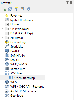
2. Go to the Browser panel. Expand the XYZ Tiles section and drag the OpenStreetMap layer to the map canvas.

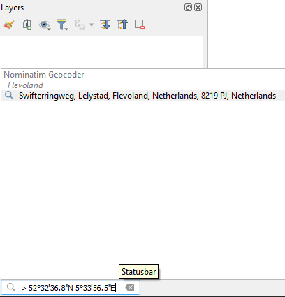
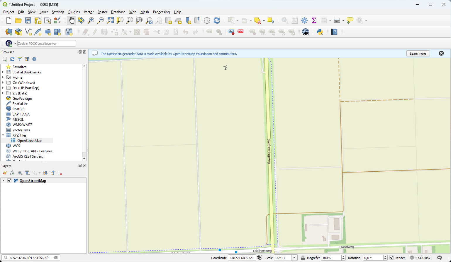
3. In the Locator bar at the bottom left, type > and a space. Then paste the coordinates mentioned above.

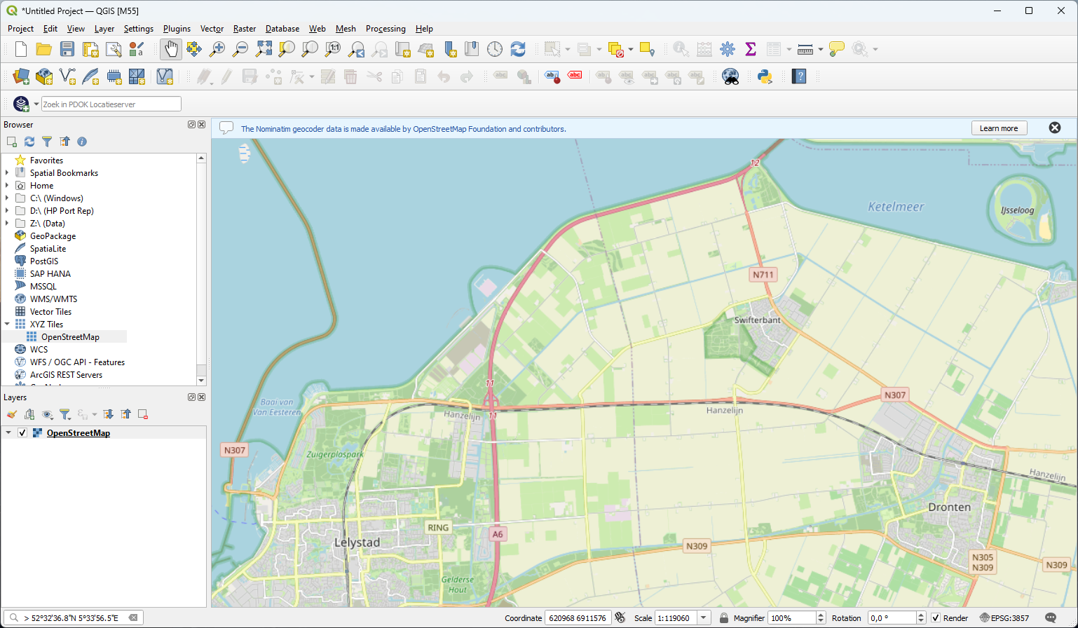
4. Click on Swifterringweg to zoom to the area.

5. Zoom a bit out so we have more context, before we're going to add open data for this area in the next sections.

We can create a Spatial Bookmark that we can use to find this extent back easily later.

6. In the Toolbar click the New Spatial Bookmark icon

7. In the Bookmark Editor, type a Name for the name of the bookmark and a Group name to organise the bookmarks in groups:

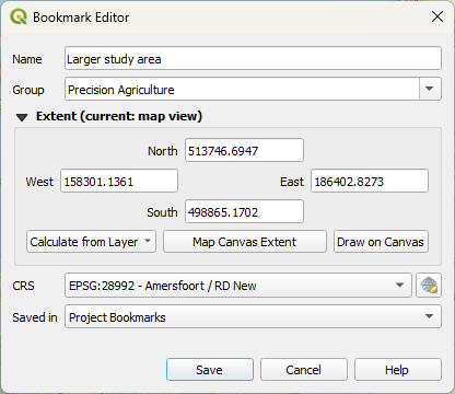
We use the Map Canvas Extent here.

You can choose to save the bookmark in your project. Then it's only available in the current project. You can also choose to save the bookmark as a User Bookmark, so it's available for all projects, because it's stored in your profile.

8. Click Save.

Let's try if this works.

9. Zoom in or out to change the extent. You can also pan to another area.

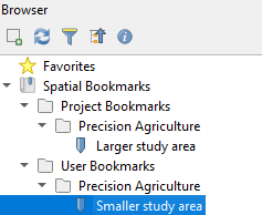
10. In the Browser panel, expand the folder Spatial Bookmarks and double-click the Larger study area bookmark.

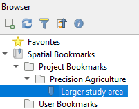
Now you're back at the defined extent.

3. Installing the PDOK Services Plugin

Open data for the Netherlands is available through PDOK. QGIS has a nice plugin to access the OGC services from PDOK: the PDOK Services plugin.

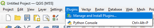
1. Install the PDOK services plugin. In the main menu go to Plugins | Manage and Install Plugins....

2. Search for the PDOK services plugin and click Install Plugin.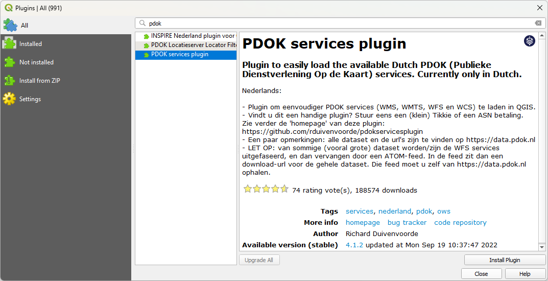

3. Click Close after successful installation.

In the next sections we're going to add open data from the PDOK services plugin to our map canvas.

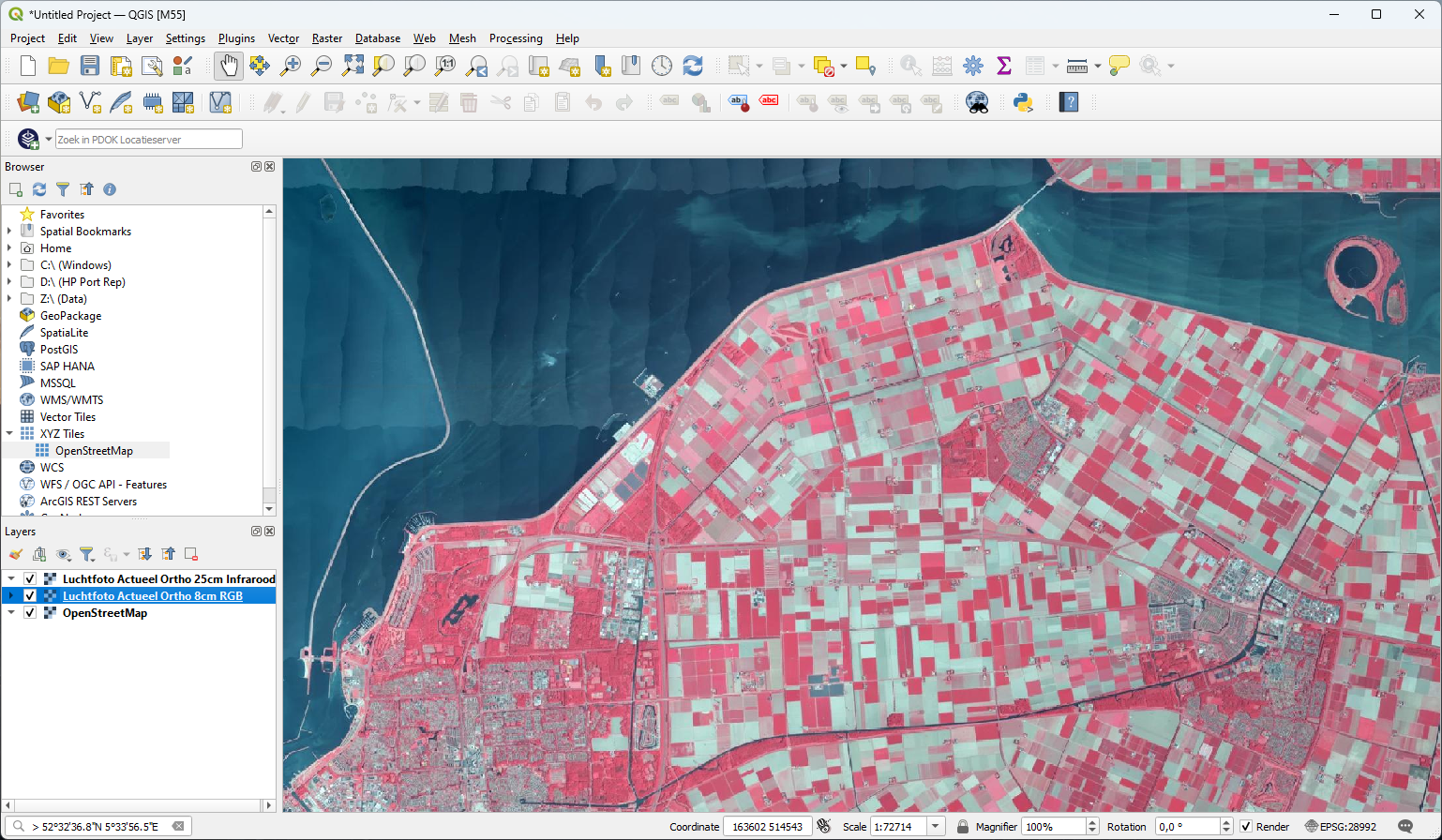
4. Add RGB and Infrared aerial photographs

To better orient ourselves, we can add aerial photographs to our project. We'll first add an RGB (red, green, blue) aerial photograph layer that gives us visual information. Next, we'll add a false color aerial photograph layer, which shows near infrared reflection in red, which is useful for detecting natural vegetation cover and crops.

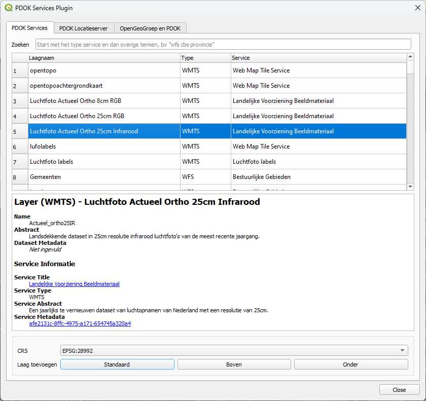
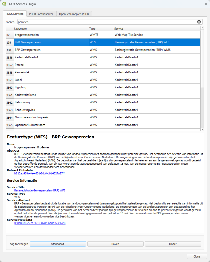
1. Click the icon in the toolbar to open the PDOK Services Plugin dialog.

The dialog is in Dutch, but is quite easy to understand:

Zoeken = search
Laagnaam = layer name
Type = OGC service (WMS, WMTS, WFS, WCS)
Service = description of the layer/service

2. Search for Luchtfoto Actueel Ortho 8cm RGB (luchtfoto means aerial photograpj) and click on the layer name.

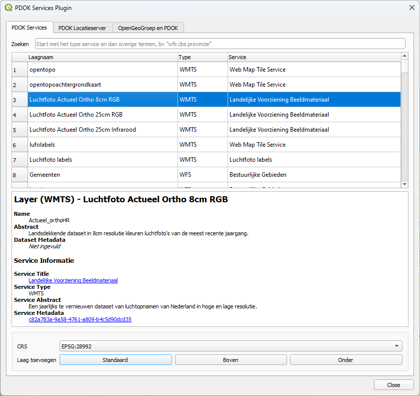
The lower part of the dialog now shows the metadata for this layer. The aerial photographs are obtained every year. This is the most recent one. Below the metadata you can choose the coordinate reference system (CRS). The default is the Dutch Amersfoort RD New projection (EPSG: 28992), which we'll also use in our project. Below the projection you can choose where in the Layers panel the layer needs to be added:

Standaard: default
Boven: add layer at top of the Layers panel
Onder: add layer at bottom of the Layers panel

3. Choose Boven to add this layer above the OpenStreetMap layer.

4. Click Close to close the dialog.

5. Change the projection of the project to EPSG:28992. You can do this by clicking right on the Luchtfoto Actueel Ortho 8cm RGB layer in the Layers panel and choose Layer CRS | Set Project CRS from Layer from the context menu.

6. Click OK in the popup to accept the default transformation setting.

5. Zoom in to our area and check the detail. You can use again the Locator bar to find the area.

6. Now repeat the procedure to add Luchtfoto Actueel Ortho 25cm Infrarood from the PDOK Services plugin to the map canvas.

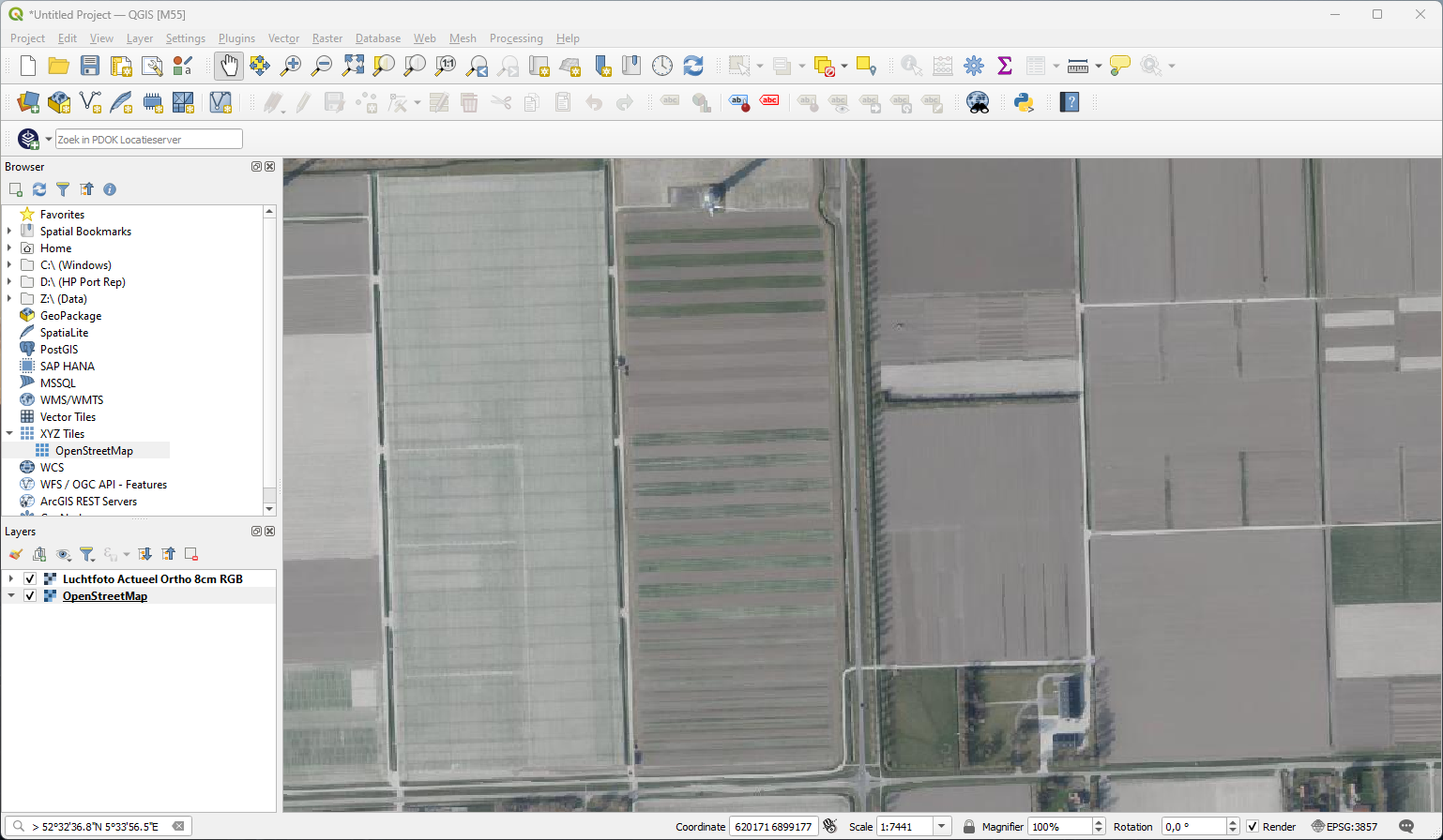
Can you see which parcels have growing crops?

7. Save your project.

In the next section we'll save these layers for offline use.

5. Save a layer for offline use

When you use your laptop in the field, you often have no internet. Therefore, it can be useful to save the online layers to your laptop. Here you'll learn three methods.

Export a rendered image
Export the map canvas
Export raster tiles

1. Zoom out to an area with multiple parcels, for example: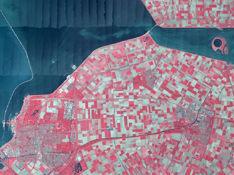

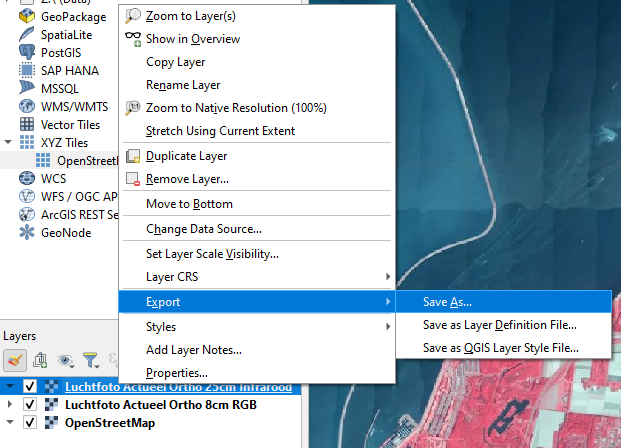
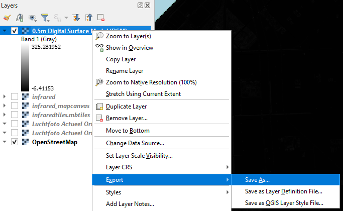
2. In the Layers panel, right-click on Luchtfoto Actueel Ortho 25cm Infrarood and choose Export | Save as... from the context menu.

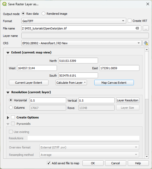
3. In the Save Raster Layer as... dialog change the output mode to Rendered image. This is needed to split the colours in the 3 RGB channels.

4. Uncheck the Create VRT box and use the button to browse to the folder where you store the data for this project and type infrared.tif as the output File name.

5. For the extent, click on Map Canvas Extent and for the Horizontal and Vertical resolution type 5 meter (we can use 0.25 m, which is the original resolution, but the file will be very large).

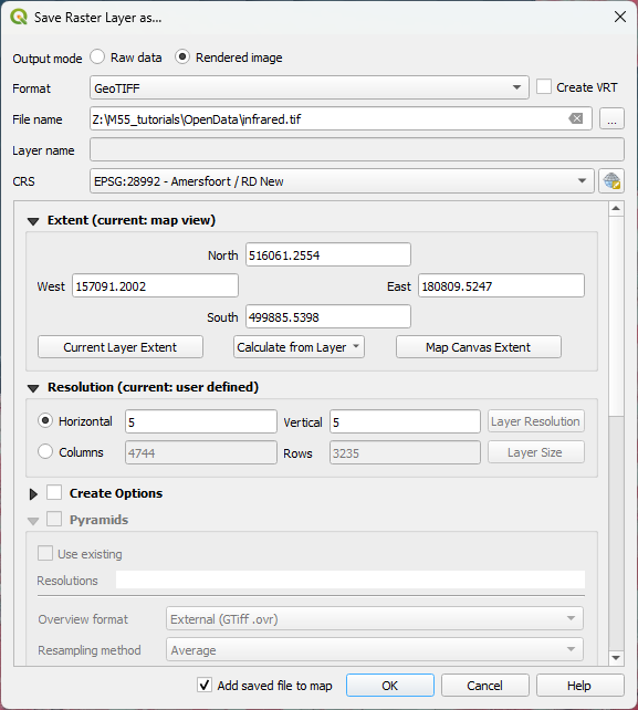
6 .Click OK to create the layer and add it to the map canvas.

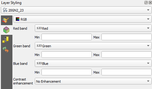
7. Click to open the Layer Styling panel and you'll see that it is now using the Multiband color renderer.

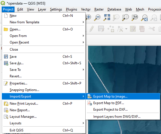
You can also save a georeferenced rendered image of the map canvas to a GeoTIFF. It will save everything visible in the map canvas to the GeoTIFF.

8. In the main menu go to Project | Import/Export | Export Map to Image....

In the Save Map as Image dialog you can set the extent, the resolution, etc. The checkbox to Append georeference information should be checked for a georeferenced image. You can also click Copy to Clipboard if you want to paste the map in a document.

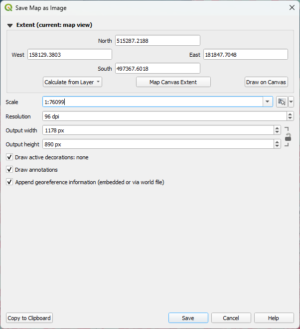
9. Click Save.

10. Save it with the name infrared_mapcanvas.tif (choose the TIF format!).

The result is not automatically added to the map canvas. You can find it in the Browser panel.

11. Drag the infrared_mapcanvas.tif layer to the map canvas to add it to the project.

12. Compare the resolution differences.

A more sophisticated way of exporting the false colour image for our area is to create raster tiles (XYZ tiles). Then tiles are generated for different zoom levels and you can keep the performance and detail for the different zoom levels.

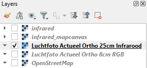
13. Make sure only the Luchtfoto Actueel Ortho 25cm Infrarood layer is selected in the Layers panel. Hide the other layers by unchecking the boxes.

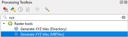
13. Click in the Toolbar to open the Processing Toolbox.

14. Search for XYZ tiles and double click on Raster tools | Generate XYZ tiles (MBTiles).

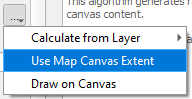
15. Choose Use Map Canvas Extent as Extent:

16. Choose a Minimum zoom of 12 and a Maximum zoom of 17. It will then generate the tiles for these zoom levels only.

17. Keep the rest as default and save the Output file to your folder with the name infraredtiles.mbtiles.

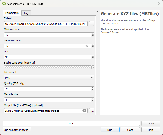
18. Click Run. Click Close when the algorithm has finished.

Also the mbtiles layer is not automatically added to your project. You can find it in the browser panel.

19. Drag infraredtiles.mbtiles from the Browser panel to the map canvas and explore it at different zoom levels.

Next we're going to explore elevation data.

6. Add a high resolution elevation layer

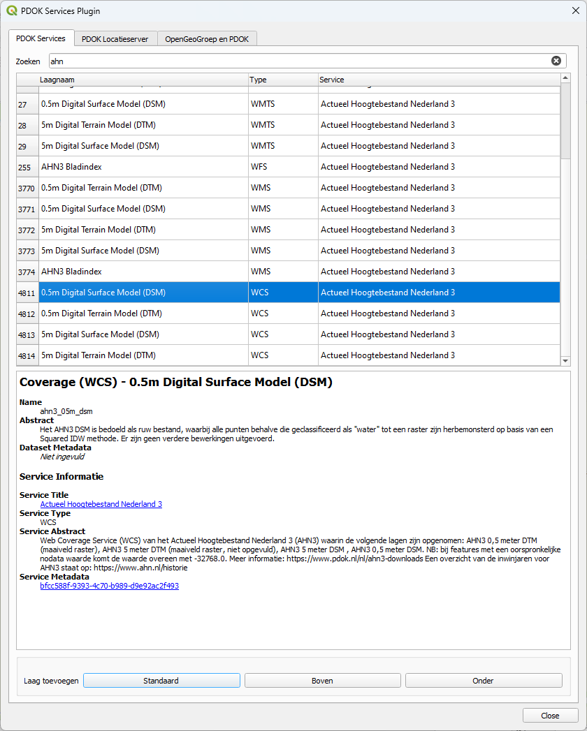
Through the PDOK Services plugin we can also add high resolution digital elevation models (DEM). We can choose between digital surface models (DSM), which has all natural and man-made objects, or digital terrain models (DTM), which has the elevation of the terrain.

1. Zoom in to an area around our study area.

2. Go to the PDOK Services plugin dialog and add the 0.5m Digital Surface Model (DSM) in WCS format

With the WCS format we get raster data that is suitable for calculations.

Let's first export the raster to a GeoTIFF that only covers our area of interest.

3. Zoom to the area of interest, a bit larger than the parcel of the coordinate.

4. In the Layers panel right-click on the 0.5m Digital Surface Model (DSM) layer and choose Export | Save As... from the context menu.

5. This time use for Output mode Raw data, choose the Map Canvas Extent for Extent and save the result in your folder as dsm.tif.

6. Click OK.

If you make the area large it can take some time. Make sure you have enough disk space for large areas.

7. Go to the Layer Styling panel. Make sure the dsm layer is the active layer and choose Singleband pseudolor as renderer.

8. Use the drop down menu at Color ramp to choose the Turbo ramp.

9. Expand the Min / Max Value Settings section and play around with the settings to get a good contrast in the parcels of our study area.

You can clearly see the trees and human-made objects. But you can also see patterns in the parcels, indicating micro relief, which affects the local drainage in the field. We can better investigate this if we look at the DTM.

10. Go to the PDOK Services plugin and load the 0.5m Digital Terrain Model (DTM) in WCS format. Then repeat the steps so we have a styled layer that we can study.

Tips:

When you export the layer choose for the extent to Calculate from layer and choose the dsm layer, so you have the same dimensions. Save the file as dtm.tif.
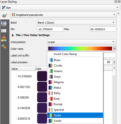
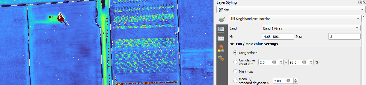
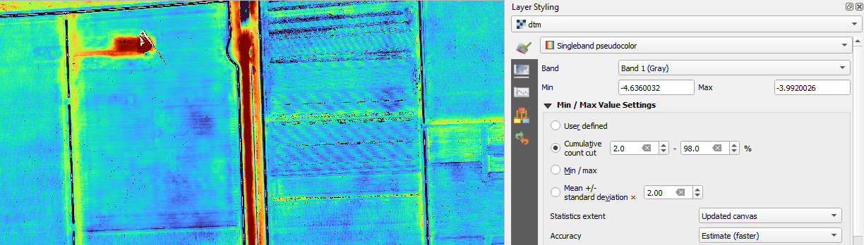
In the Layer Styling panel try to change under Min/Max Value Settings the Statistics extent to Updated canvas. The colours will then be stretched to the min/max values of the map canvas, everytime you pan.

We can even get more detail when we download point cloud data, which we'll do in the next section.

7. Add point cloud data

In this section we'll add point cloud data to our project. We'll use the AHN4 LiDAR data for the Netherlands.

1. In your webbrowser, go to GeoTiles.nl.

2. Find the tiles that cover our study area.

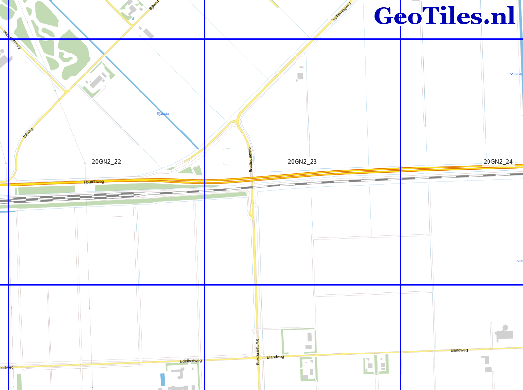
We need to download multiple tiles. Let's start with tile 20GN2_23.

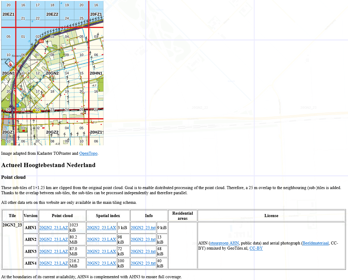
3. Click on tile 20GN2_23.

4. Download the 20GN2_23.LAZ file. LAZ is a point cloud format, supported by QGIS through the PDAL library.

5. After downloading locate the LAZ file in the QGIS Browser panel and drag it to the map canvas.

While QGIS is converting the file it will show the extent:

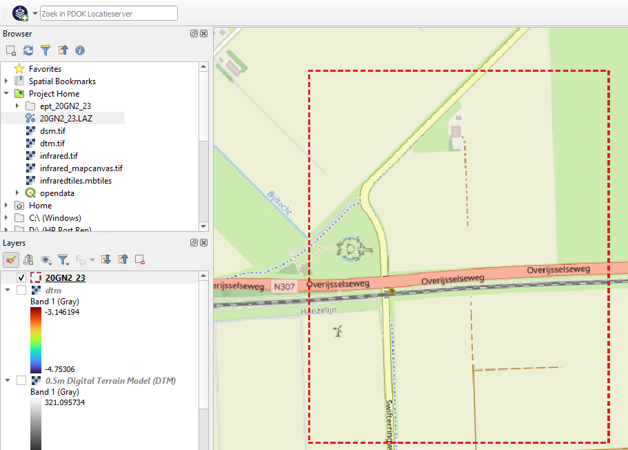
After processing, it will show the points with the RGB colors:

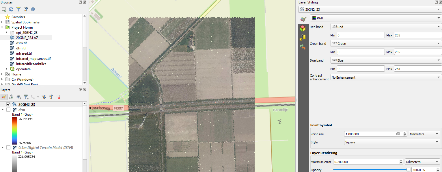
In the Layer Styling panel you can also choose other attributes of the point cloud layer.

6. Try:

Classification
Attribute by ramp with different settings

A much nicer way to look at point clouds is to use the 3D view.

7. Make sure that in the Layer Styling panel the 3D View tab is set to RGB. In that way we can see the points with the RGB colours in the 3D view.

8. In the main menu, go View | New 3D Map View.

Tips:

QGIS 3.28 or newer gives some more settings
Use the aerial photograph in RGB as a background
Download the other tiles and repeat

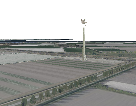
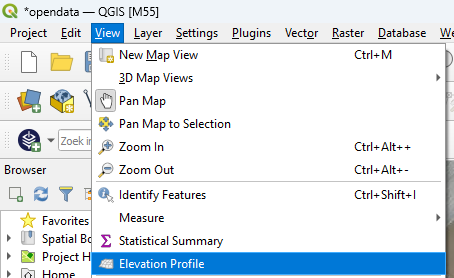
In QGIS 3.28 or newer you can explore the profiles in an easy way.

9. In the main menu, choose View | Elevation Profile.

A new panel opens at the bottom of the QGIS window.

10. In the Elevation Profile panel, click the Capture Curve icon and draw a transect. With right-click you end the transect and it will show up in the panel.

11. Click the Options icon and increase the Tolerance to 25 meter.

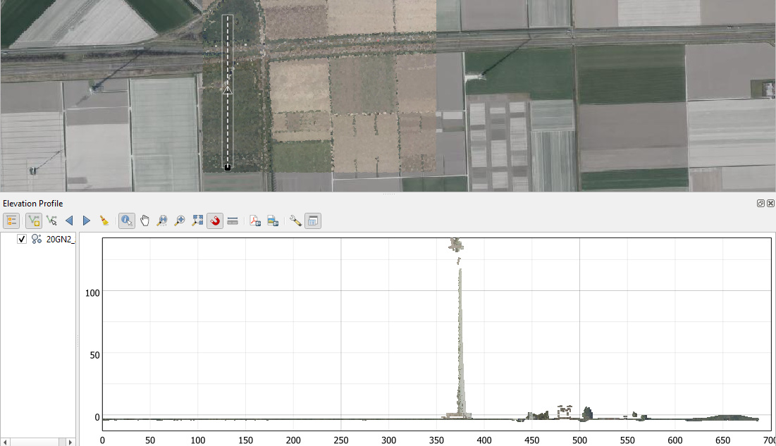
Zoom in and play with the tolerance to see what's in the scene.

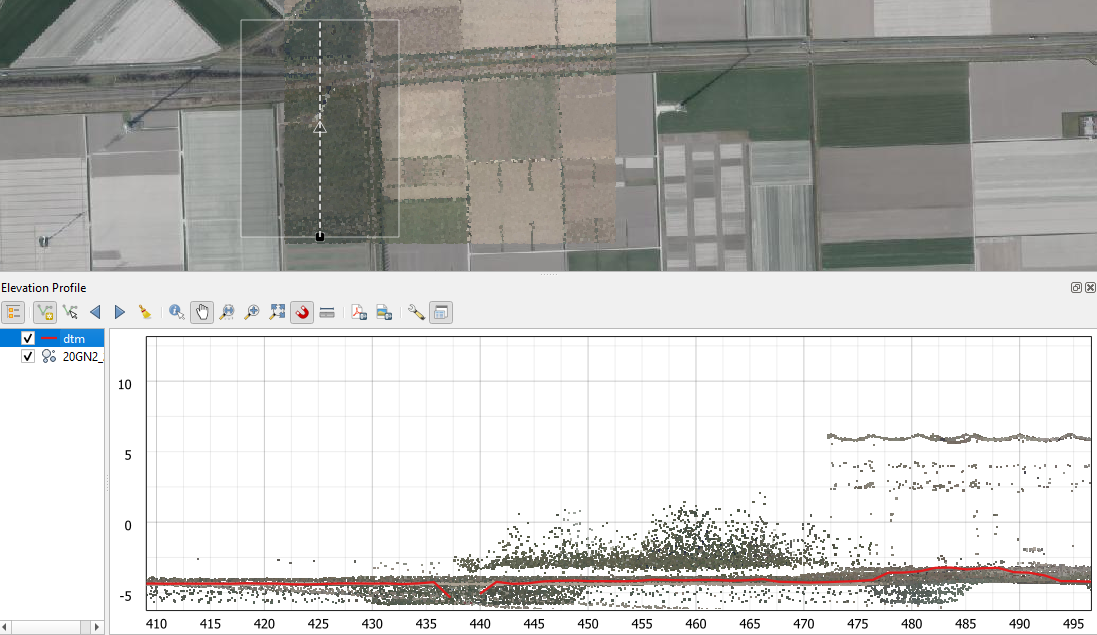
You can use also other layers that have elevation information, like our DTM and DSM.

12. In the Layers panel right-click on the dtm layer and choose Properties... from the context menu.

13. In the Layer Properties dialog, go to the Elevation tab and check the box before Represents Elevation Surface and click OK to close the dialog.

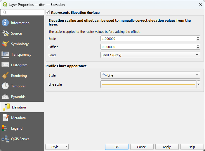
Now the dtm layer is also added to the profile panel.

More resources about point clouds are in this playlist:

8. Add parcel polygons

A very useful dataset for agricultural applications is a crop map. For the Netherlands there's a parcel map with crop data available every year and we can load it through the PDOK Services plugin.

1. Go to the PDOK Services plugin dialog.

2. Look for the layer BRP Gewaspercelen in WFS format and add it to the map canvas. Make sure you're zoomed in to the area of interest, because the layer is very large to load.

3. Export the polygons for the area of interest. In the Layers panel, right-click on the BRP Gewaspercelen layer and choose Export | Save features as... from the context menu.

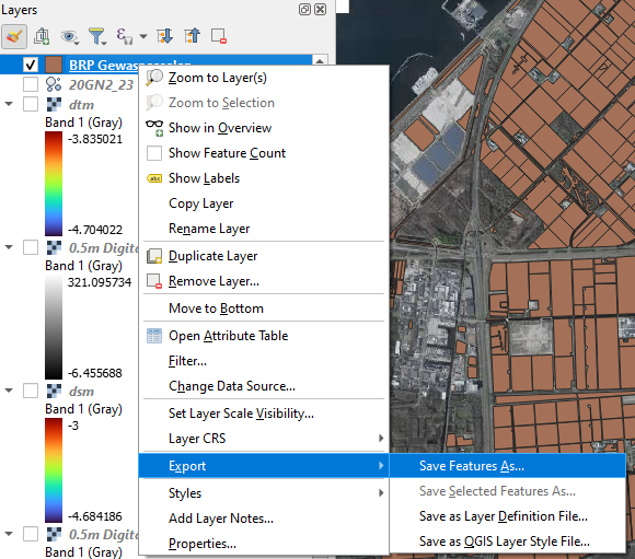
4. Let's save it to a GeoPackage with the name farmdata.gpkg and the layer name parcels. Under extent use the extent of the dsm layer again.

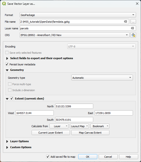
5. Click OK.

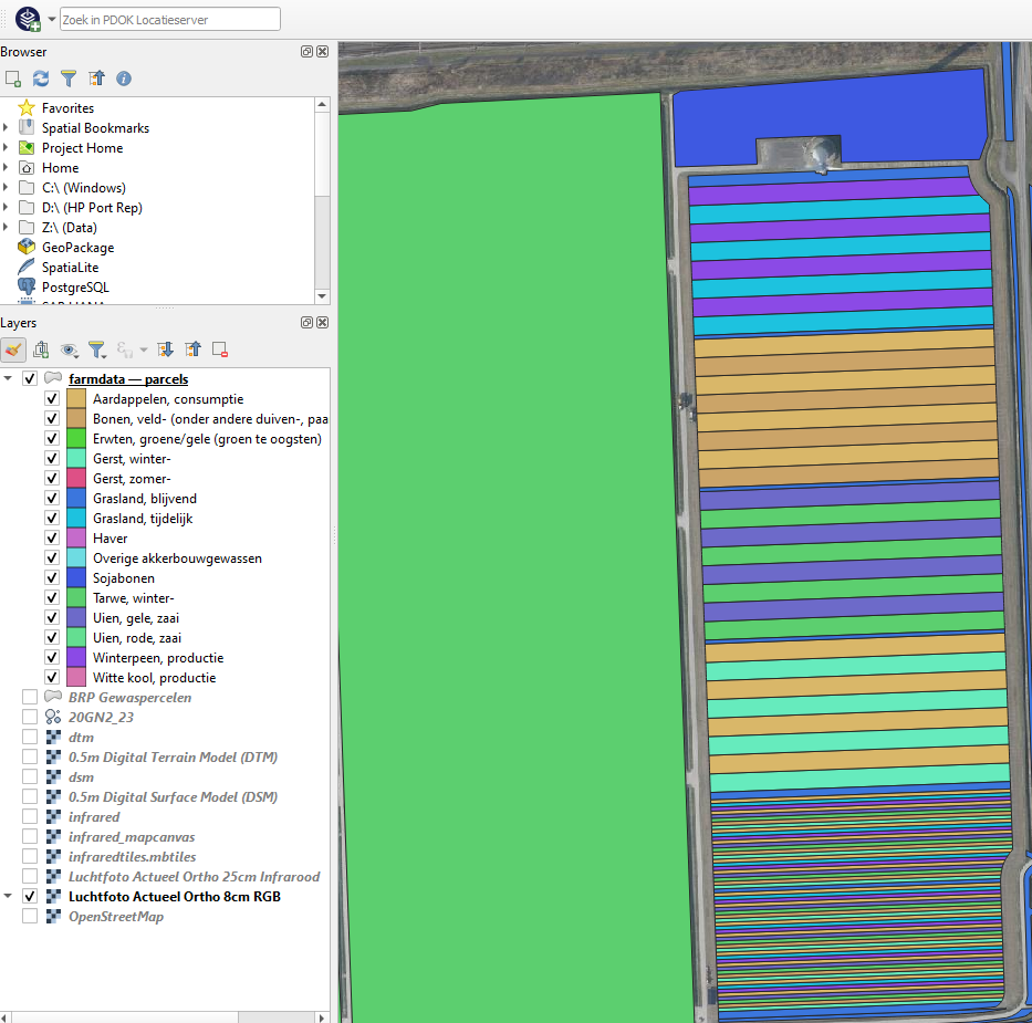
Let's style the layer so we can distinguish the different crops.

6. Go to the Layer Styling panel and make sure that the parcels layer is active.

7. Change the renderer from Single Symbol to Categorized.

8. For Value choose gewas, which means crop type and click Classify.

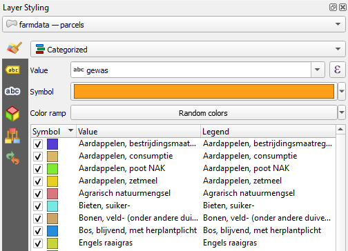
Which crops do you see in our study parcels? Translate them to English.

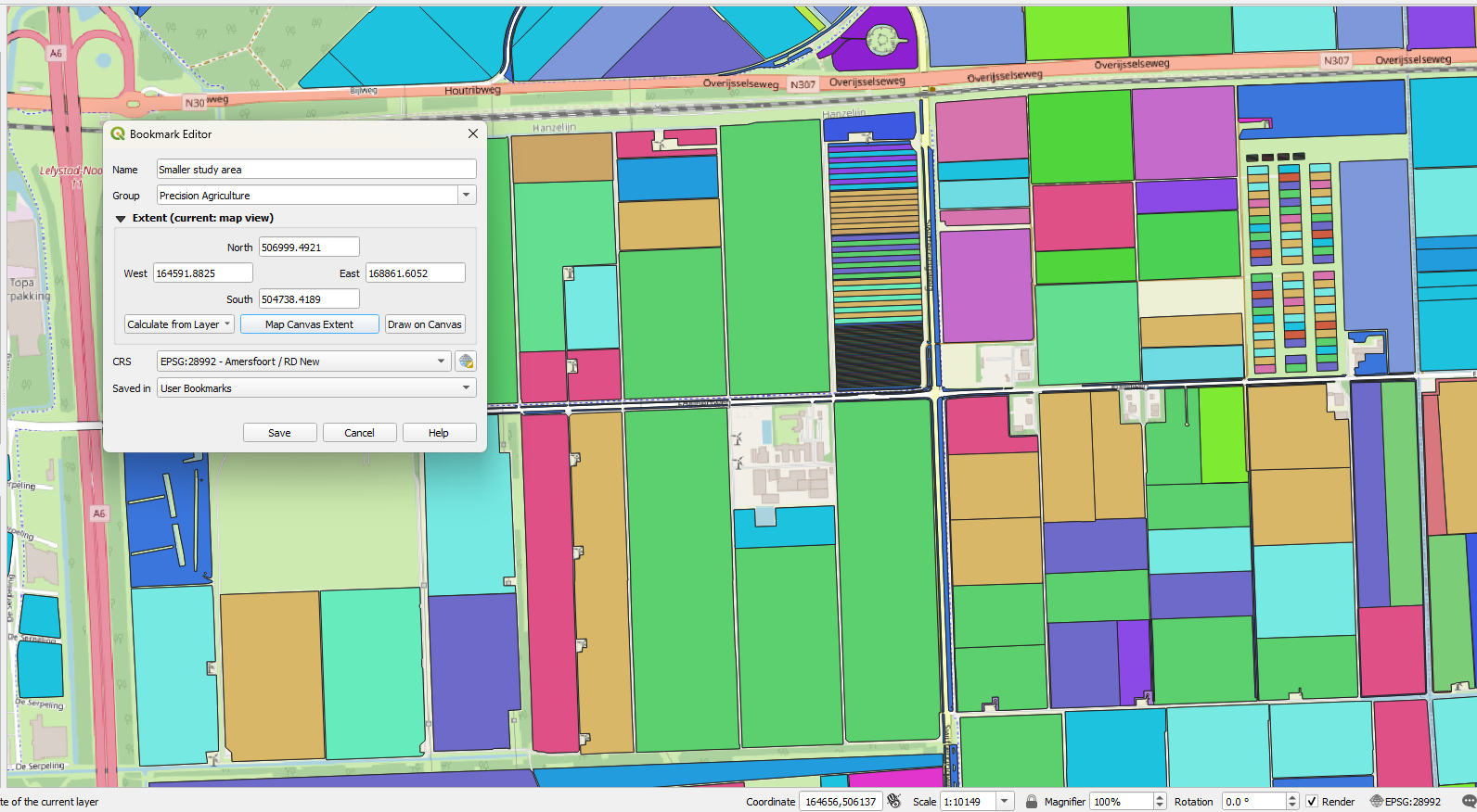
Tip: in the Layers panel you can show the legend for the visible part of the layer only:

9. Create a Spatial Bookmark for the Smaller study area. This time save it in your User Bookmarks, because we need it later in another project. Use approximately the area below.

In the next section we'll add a soil map.

9. Add soil data

Soil maps also provide important information for agricultural applications. Let's load one through the PDOK Services plugin.

1. Go to the PDOK Services plugin dialog and add the Bodemvlakken layer, which is only available in WMS format.

2. Duplicate the parcels layer: right-click on the layer name in the Layers panel and choose Duplicate Layer from the context menu.

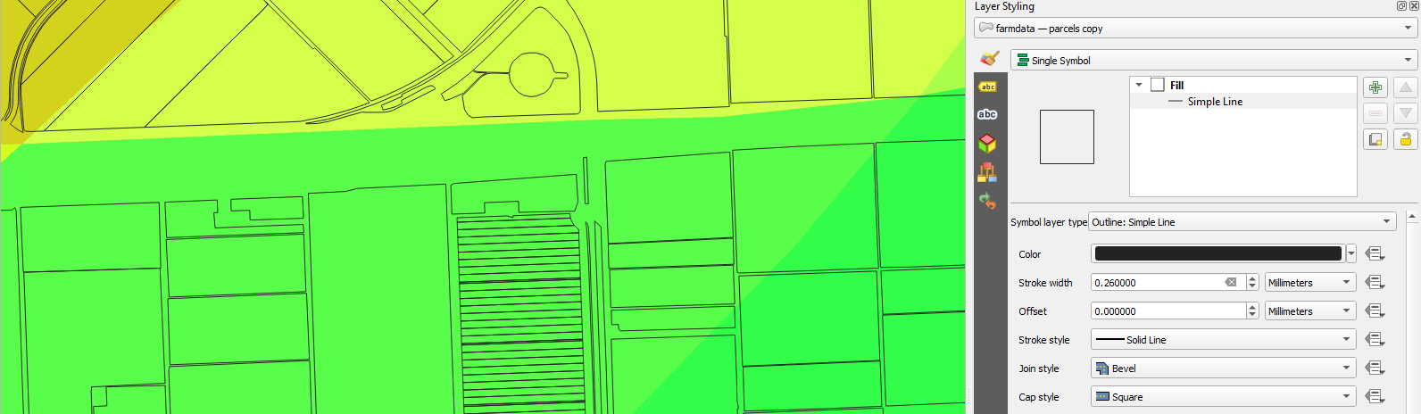
3. Hide the parcels layer and in the Layer Styling panel make sure that the parcels copy layer is active.

4. Change the renderer back to Single Symbol.

5. Click Simple Fill and change the subrenderer to Outline: Simple Line. Make sure there's now a thin black line around the parcels.

Now you can check the soil types.

Which soil classes are in the study area?

10. Conclusion

In the Netherlands, many high resolution datasets are freely available through the PDOK Services plugin. You have learned how to add layers to your project and to save them to your harddisk.

For areas with less data availability, you can use global open datasets or derive them from satellite imagery. Often these datasets have a much lower spatial, temporal and/or thematic resolution.

Open data resources can be found here. They can often be added through OGC standards. Watch this playlist to learn more about data sharing and using open data in QGIS: