The Michel-Lévy Interference Color Chart – Microscopy’s Magical Color Key
Editor’s Note:
The figures in this article are included to support the text and are intended for online viewing only. We make no claims to the accuracy of the colors or readability of the charts online or if printed due to the wide variety of monitors and printers available for use today. Print versions of the Michel-Lévy charts are available as referenced in this article as well as from several microscope manufactures and their representatives.
Download the PDF version of “Using the Michel-Lévy Color Chart”.
The Michel-Lévy interference color chart has been in continuous use by analytical microscopists for more than 100 years. Why such endurance? Because this chart, also known as the Michel-Lévy Table of Birefringence, is just as useful today as it was over a century ago in unlocking the many mysteries of microscopic particle analysis and identification. This extraordinarily valuable aid to the polarized-light microscopist graphically relates the thickness, retardation (optical path difference), and birefringence (numerical difference between the principal refractive indices) for particular views of transparent, colorless or colored substances. These characteristics allow unknown materials to be identified; additionally, they provide important optical information about those materials whose identity is known.
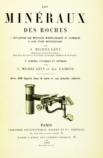
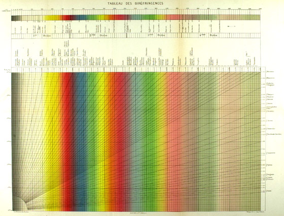
The Michel-Lévy interference color chart was first introduced to the world in a book published in Paris in 1888 (1). This book (Figure 1) was called Les Minéraux des Roches, and was devoted to the subject of rock-forming minerals. In Part I, Auguste Michel-Lévy (1844–1911) described the methods used by mineralogists and chemists in the microscopical study of minerals, and, in Part 2, Michel-Lévy, together with Alf. Lacroix, tabulated the physical and optical properties of the rock-forming minerals. Michel-Lévy acknowledges the work of previous investigators, including his friend and mentor (“mon maître et ami”) F.A. Fouqué, with whom he had collaborated in the production of the two-volume, Minéralogie Micrographique; Roches éruptives Françaises (1879), with its beautiful atlas of 55 chromo-lithographed plates; Des Cloizeaux, Manuel de Mineralogie (1862); Mallard, Traité de Cristallographie (1884); DeLapparent, Cours de Minéralogie (1884); and even Rosenbusch, whose second edition of Mikroskopische Physiographie had come out in 1885; Klement and Renard’s Reactions Microchimiques (1886) and their predecessors are acknowledged for their microchemical contributions. But now, in this 1888 book, we see in color, for the first time, Michel-Lévy’s “Tableau Des Biréfringences” (Figure 2). The chart is a large (about 24″ X 18″) chromo-lithograph based on a water-color original; it folds in half, bottom-to-top, and then folds four times, accordion-like, and is tipped in at the back of the book. It is rare to find these charts that are not in need of some repair, as the paper quality was not good, and they cannot now take repeated folding and unfolding. We will come back to this chart’s history, and to the others which followed it, presently.
The early applications of the Michel-Lévy interference color chart were in the fields of mineralogy and petrology, for the identification of mineral grains in rock thin-sections, and also for comminuted, free mineral grains. The general utility of the chart, however, is such that today it is used as an aid not only for the identification of minerals, but synthetic textile fibers, chemicals, food and food-processing ingredients, biologicals, drugs, catalysts, ores, fertilizers, explosives, etc., etc. In fact, the chart is today used routinely by analytical microscopists in the identification of almost all dust-size particles regardless of nature or origin; it is fundamental to the use of The Particle Atlas (2). Some specific fields of application include criminalistics (trace evidence analysis), air pollution, pharmaceuticals, aerospace, papermaking, microelectronics, fibers, polymers, explosives, manufacturing, graphic arts, and brewing!
What about the “interference color” in the name of the chart? Colors due to the interference effects of light are commonly seen in soap bubbles, oil films or slicks, and between two pieces of glass that are stuck together (separated by a very thin layer of air). These colors are often mistakenly referred to as “rainbow” colors; they are, in fact, not solar spectral colors at all (notice the magentas, grays and white in a thin layer of oil on water next time you see an oil slick). The same kinds of interference colors seen in soap bubbles and oil films are seen in most microscopic particles, when the observation is made with a polarized-light microscope. The polarized-light microscope – the principal investigative instrument for the observation of these interference colors – is, essentially, a conventional microscope with the addition of polarizing elements above and below the specimen, usually in the “crossed” position, i.e., with their “preferred vibration directions” perpendicular to one another. The lower polarizer, or “polar” as it is familiarly referred to by those in the field, is usually oriented in the microscope so that its vibration direction runs “East-West” (left-right; 3 o’clock-9 o’clock); the upper polarizer, called the “analyzer,” is oriented so that its vibration direction runs “North-South” (12 o’clock-6 o’clock). The vibration direction of any polarizer may be determined by viewing reflections from a horizontal, non-metallic surface through the polarizer. All such reflections have their polarization oriented horizontally, i.e., “East-West.” View a reflected highlight on a horizontal shiny non-metallic surface through the polarizer while rotating it. The reflection will be seen to disappear twice on complete rotation of the polarizer; in these positions, the vibration direction of the polarizer is “North-South,” canceling the “East-West” reflection polarization. Try this with a pair of polarizing sunglasses, whose vibration directions are, of course, oriented “North-South” (i.e., up-and-down) to eliminate, or cancel out, the natural “East-West” (left-right) orientation of light reflected from water, glass, and other shiny, non-metallic surfaces.
Any bio-medical type microscope can be converted for interference color observation by placing one polarizing element, the “polarizer,” anywhere below the specimen in the light path, such as over the light exit port, in the filter carrier, between the lenses of the condenser, on the top lens of the condenser, but not too near the light source. Orient the polarizer vibration direction “East-West.” The second polarizing element, the “analyzer,” is placed in a “crossed” position anywhere above the specimen, such as on the back of the objective, in the eyepiece, on the eyepiece diaphragm, or on top of the top (eye) lens of the eyepiece. Orient the analyzer vibration direction “North-South.” But a true polarized-light microscope with graduated, rotating polars; graduated, rotating stage; slot for accessory plates; Bertrand lens; and other features is necessary for more advanced, quantitative optical crystallography.
Attend an online course in Polarized Light Microscopy offered by Hooke College of Applied Sciences, a member of The McCrone Group.
![]()
Color Where There is None
If you were to take all transparent substances in the world, natural or man-made, and view them between crossed polars using a polarizing microscope, and then view them in all possible orientations, you would observe one of two effects: either the specimen will show interference colors, and appear bright and colored against a black background, or it will not be seen at all; i.e., the field remains black.
Substances which remain dark at all orientations between crossed polars are called isotropic. The term “isotropic” means the “same velocity,” and refers to the fact that light travels through the substance at a single velocity, regardless of direction; the numerical value of any measured property will be identical along any direction in which it is measured. Such substances are either amorphous (e.g., glass), or they belong to the cubic crystal system and have just one refractive index. About 5%-7% of transparent solids fall into this category, and to identify these substances it is only necessary to determine the specific value of the characteristic refractive index (usually done with the Becke line by the immersion method, in which the isotropic substance is successively immersed in liquid media of known refractive index until one is found in which the substance disappears when viewed with monochromatic light), and look up the value found in reference books where such data are tabulated. Examples of isotropic substances are common table salt, glass, diamond, silver chloride, mineral wool, fiberglass, and unoriented polymers.
Substances which appear bright with interference colors on a black background are termed anisotropic, which means “not the same velocity;” different properties in different directions; i.e., different refractive indices along the different axes. Anisotropic substances fall into two major groups – those having two principal refractive indices, and those having three principal refractive indices.
Anisotropic substances having two principal refractive indices, epsilon (ε) and omega (ω) belong to the tetragonal or hexagonal crystal systems. Crystals in these two systems have one unique view, along which they appear isotropic; thus they are termed uniaxial. Examples of substances having two principal refractive indices include quartz, calcite, silicon carbide, and man-made polymer fibers.
Substances having three principal refractive indices, alpha (α), beta (β), and gamma (γ), belong to the orthorhombic, monoclinic, or triclinic crystal systems. Crystals in these three systems have two views along which they appear isotropic; thus they are termed biaxial. Examples of biaxial substances include borax, talc, sucrose, mica, gypsum and oriented polymer films.
The refractive indices are characteristic identifying properties of transparent substances. It is these anisotropic substances which can be identified with the aid of the Michel-Lévy interference color chart, often without having to determine each principal refractive index individually.
The characteristic birefringence of a given substance is the numerical difference between the maximum and minimum refractive indices, that is, (ε-ω) for uniaxial substances and (γ-α) for biaxial substances. We can designate birefringence generally as (n2-n1). Only in particular orientations of a crystal do we see the characteristic birefringence γ-α for biaxial and ε-ω for uniaxial crystals; n║-n┴ for polymer fibers and n║ (machine direction) – n (┴ to film) for polymer films. All other orientations show lower values of n2-n1.
Isotropic substances do not have a birefringence, because they possess only a single refractive index; there can be no numerical difference.
In 1889, Michel-Lévy and Lacroix published a set of tables (3) listing the birefringences and other optical and physical characteristics of rock-forming minerals.
Destructive Interference Does It
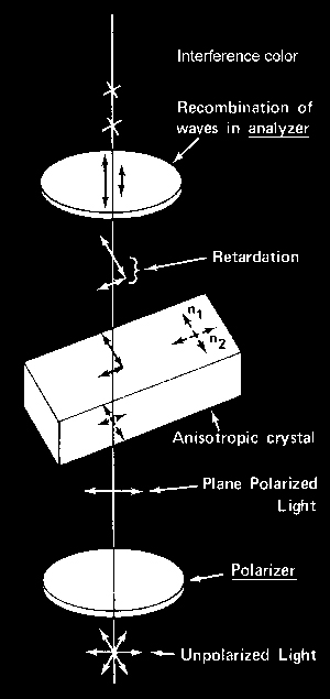
Let’s see what happens to light as it passes through a polarizer, an anisotropic crystal oriented at 45° to the crossed polars, and through the analyzer – refer to Figure 3. Unpolarized light vibrating in many different planes enters the polarizer, and is rendered plane-polarized; i.e., all of the light that passes through the polarizer (about 32-37%) is vibrating “East-West.” On entering a doubly refractive (anisotropic) substance, the plane-polarized light is immediately resolved into two mutually perpendicular rays, each traveling through the crystal at different velocities, n1 and n2; one travels slowly (high refractive index direction) and one travels fast (low refractive index direction); how fast or slow depends on the atomic structure. Light travels through crystals in mutually perpendicular directions; only two directions will be viewed at any one time in the microscope; the third will be parallel to the microscope axis. Since each of the two rays passes through the crystal at a different velocity, the fast ray will emerge from the crystal before the slow ray does. With both rays out of the crystal, there will be a path difference between the two, which is known as the retardation, i.e., the slow ray is retarded with respect to the fast ray. This retardation distance for microscopic crystals is very small, and is measured in nanometers (nm). A single nanometer is one one-millionth of a millimeter (the old name for nanometer was millimicron); 1 nm = 0.001 µm = 0.000001 mm.
When the two rays enter the upper polarizer, they are recombined vectorially (vectorially analyzed; hence “analyzer”), and the retardation, a phase shift, results in destructive interference for certain wavelengths to give the interference colors we see when we use crossed polarizers.
Interference colors vary in hue with the retardation according to a characteristic sequence, known as Newton’s series (the same colors seen in soap bubbles). Newton’s colors are not those of the solar spectrum, or those seen in the rainbow, remember. They are the colors that Newton observed when he pressed together two plates of glass which were not perfectly true planes. The colored rings which were produced were described by him in Book II, Part I of his Opticks, and divided into the following orders:
-
-
- Black, blue, white, yellow, red
- Violet, blue, green, yellow, red
- Purple, blue, green, yellow, red
- Green, dirty red
- Greenish blue, red
- Greenish blue, pale red
- Greenish blue, reddish white
-
Since Newton’s time, the interference color scale has been worked out in great detail, and the numerical values for the retardations and the air film thickness necessary to produce them were determined during the period 1854-1902. The values obtained and the verbal descriptions of the colors may differ with each researcher because the positions of the different bands vary somewhat for different sources of illumination. For example, the value for the retardation of the so-called “sensitive violet” is given by both Wertheim (4) and by Quincke (5) as 575 nm, by Rollet (6) as 556 nm, and by Kraft (7) as 535.6 to 557.6 nm for clear sky. Kraft’s values varied so because he found that the same retardation produced different colors when the method of illumination was changed from Argand or incandescent electric light, to Auer burner, to electric arc, to snow illuminated by the sun, to gray, cloudy sky, to clear sky! Other factors which will also cause differences in perceived colors include no daylight blue viewing filter in the light path, a daylight filter which is too blue, and a lamp rheostat which is turned down too low. The values and colors used in most petrographic textbooks, and in the popular Zeiss Michel-Lévy Color Chart (Figure 4), with small changes, are those of Quincke (8). Newton’s Color Scale, as modified from Quincke, consists of the following values and colors between crossed polars up to the first order:
|
Retardation (nm)
|
Order
|
Interference Color
|
|||
| 0 | 0 | Black | |||
| 40 | Iron-gray | ||||
| 97 | Lavender-gray | ||||
| 158 | ¼ | Grayish-blue | |||
| 218 | Clear gray | ||||
| 234 | Greenish-white | ||||
| 259 | Almost pure white | ||||
| 267 | Yellowish-white | ||||
| 275 | Pale straw-yellow | ||||
| 281 | Straw-yellow | ||||
| 306 | ½ | Light yellow | |||
| 332 | Bright yellow | ||||
| 430 | Brownish-Yellow | ||||
| 505 | ¾ | Reddish-orange | |||
| 536 | Red | ||||
| 551 | Deep red | ||||
| 565 | Purple | ||||
| 575 | Violet | ||||
| 589 | 1 | Indigo | |||
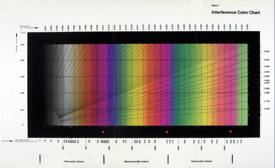
The interference colors are divided into “orders,” with the end of each order marked by a red color representing one full wavelength retardation.
The first order starts with black (retardation = 0), and for the first 250 nm or so, the intensity of all wavelengths in white light is almost uniformly reinforced, resulting in hues of gray and white. This is followed by yellow and orange hues, and ends with the very important, intense, narrow “first-order red” at about 550 nm.
The second order has intense blue, green, yellow, orange, and, finally, red hues at about 1,100 nm. Successive orders become paler and paler; the fourth to 10th orders show only a diminishing pink and green. Above about 10th order, we have only “high-order white.” Detailed treatment of the mechanism of interference color production can be found in standard references on optical crystallography (9-14).
Today, the values adopted for first-order red and the quarter-wave plate differ somewhat among the manufacturers: one manufacturer uses, respectively, 551 nm and 138 nm; other manufacturers use 530 nm and 147.3 nm, etc. Incidentally, Quincke’s Table also listed the interference colors as seen between parallel polarizers. These essentially complementary colors are useful to the advanced worker in zeroing in on a retardation value – much as annular-stop dispersion-staining colors are useful in determining more precise central-stop colors. For a discussion of parallel polarizers, see reference 15.
Retardation All Adds Up
Retardation, r, increases linearly with both the thickness, t, of a specimen and with the birefringence, n2-n1: the greater the thickness, the greater the retardation (the thicker the crystal, the farther behind the slow ray gets from the fast ray); the greater the difference between the refractive indices (birefringence) to begin with, the greater the retardation (or higher the interference color). That is,
r = t(n2-n1)
Or, let’s shorten it by putting in “B” for the birefringence (n2-n1),
where r is the retardation expressed in nanometers, nm; t is the thickness, which we measure with our eyepiece micrometer, and express in micrometers, µm; and B is the birefringence (the numerical difference between the principal refractive indices), which is unitless. It will be seen immediately that, in order to achieve equality of units, the thickness, t, must be multiplied by 1000 (1000 nm/µm) in order to express retardation in nanometers,
By transposition, we may solve for either t or B,
|
t =
|
|
|
B =
|
|
Normally, we don’t have to calculate thickness; we just use our eyepiece micrometer for the task. Likewise, we don’t normally have to calculate retardation, because we can compare the interference color we see in the microscope with the interference colors on the Michel-Lévy chart, and read it off. It’s the birefringence that we are after; that’s the identifying characteristic. Take the common mineral quartz, for example; its thickness will vary from grain to grain, and so its interference color will vary from one thickness to another; but the birefringence (the numerical difference between the principal refractive indices) is a constant; 0.009 in the case of quartz. There it is…..get the birefringence, and you may not need any other information. The Michel-Lévy chart is a rapid way of determining birefringence from the particle thickness and the maximum interference color it is displaying. The chart is a graphical solution to the above equations.

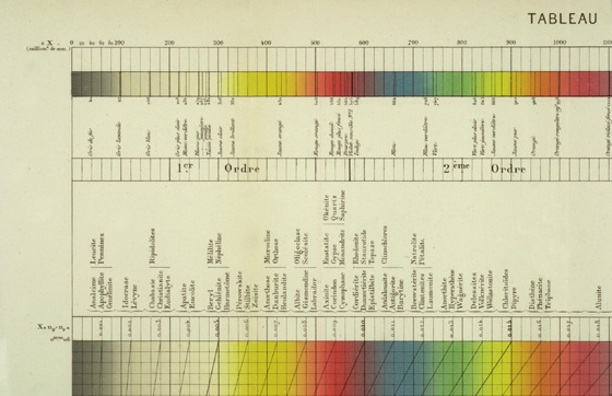
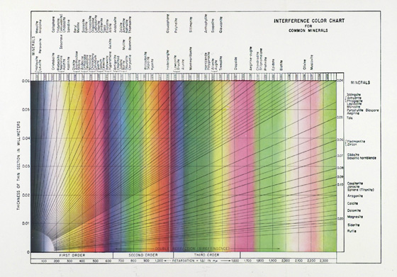
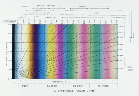
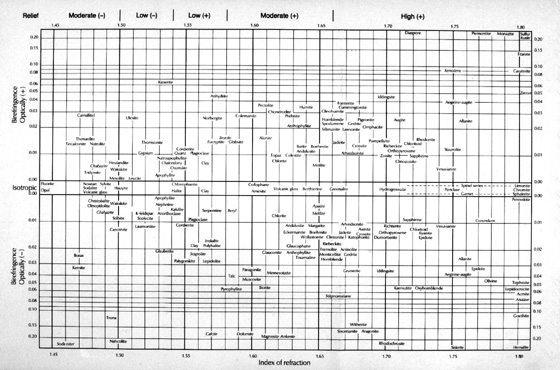
Let’s look a little more closely at the Zeiss rendition of the Michel-Lévy chart – Figure 4. Notice that the thickness, t, increases along the ordinate on the left side of the chart from 0 µm to 50 µm, and is numbered at 10 µm intervals. Along the bottom of the chart, left to right, the path difference, or retardation, r, increases from 0 nm to over 1744 nm, and is marked at specific values of retardation, 0, 40, 97, 158, 200, 218, 234 …… 1744nm (this chart uses the older designation millimicrons, mµ, for nm). The names of the interference colors are also given. First-order red falls at about 550 nm; second-order red at two times 550, or 1,100 nm; third-order red at three times 550, or 1,650 nm, etc. The birefringence (n2-n1) is plotted along the top and right side of the chart; it starts at zero at the upper-left corner, and proceeds to the right 0.001, 0.002, 0.003, 0.004 …… to 0.036 at the upper-right corner, and then proceeds downward, graduated differently, 0.040, 0.045, 0.050, 0.055 …… down to 0.180, and beyond.
Notice the family of diagonal lines originating at the lower left and going out to each value of birefringence. The diagonal lines represent the birefringence values, because t = r/B is the equation for a straight line through the origin of the coordinates with a slope of tan θ = 1/B. Each line is assigned an angle θ, and thereby a special value B. The names of many substances appear opposite their characteristic maximum birefringence value on many versions of the chart. On this Zeiss chart (Figure 4), minerals are listed by their identifying birefringence. We mentioned quartz earlier; its name is listed at 0.009; spodume is at 0.020; olivine is at 0.036; calcite is near the bottom-right of the chart, near 0.180 – a high birefringence; a large numerical difference between its refractive indices (omega = 1.6584; epsilon = 1.4864; 1.6584 – 1.4864 = 0.1720).
Know Two, Find the Other
Since the Michel-Lévy chart shows the interrelationships between thickness, birefringence, and interference color, the microscopists can, as suggested earlier, determine any one from the chart if they know the other two. Several examples will illustrate this:
Example 1: Suppose a cylindrical synthetic fiber 15 µm in diameter shows a maximum interference color corresponding to about 900 nm. This is determined by orienting the length of the fiber at 45 degrees to the vibration directions of the crossed polars, and comparing the color running down the center of the fiber to the colors in the chart. The order is found by noting the number of reds between the center and either edge of the fiber. One must be very careful here because the colors are very, very close together at the edge of a cylindrical fiber. It is often better to count orders on a taper-cut end of a fiber. In the present example, we pass through only first-order red, indicating the yellow at the center is second order.
To determine the birefringence, we look for 900 nm on the abscissa and move vertically until we reach a horizontal line corresponding to a thickness of 15 µm on the ordinate. There will be a diagonal line where the two lines intersect. We now follow the diagonal line to the upper right to read the birefringence, 0.060, at the top of the chart. Looking up this value in a birefringence table for synthetic fibers, we learn that a cylindrical fiber having this birefringence is nylon. We could also have calculated birefringence from (n2-n1) = r/1000t:
(n2-n1) = r/1000(t) = 900/1000(15) = 0.06
Remember, the 1000 in the equation is a units conversion factor between nanometers (retardation) and micrometers (thickness).
Note that the thickness of a substance, such as a crystal or fiber, must be measured along the same direction the retardation is measured. This works well for cylindrical fibers, as in the example above, since the measured diameter is also the thickness. The proper thickness for non-cylindrical specimens often can be measured by “crystal-rolling.” To do this, the specimen must be mounted between slide and cover glass in a viscous liquid such as Aroclor 1260 (Monsanto), Karo Corn Syrup, or any mounting medium having the consistency of molasses. Sliding the cover glass with a dissecting needle rolls the crystal 90 degrees to a position where the thickness can be measured directly with a calibrated eyepiece micrometer.
Some non-cylindrical fibers and polymer films can be cut with a razor at a precise 45 degree angle and the thickness measured as the horizontal projection of the cut. Polymer films can be measured directly, using a thickness gauge before mounting.
For substances having oblique extinction, the 45 degree position to the polarizer vibration direction needed before determining the interference color is quickly found with many polarized-light microscopes through the use of the “45 degree click-stop lever.” The stage is rotated until the specimen goes to extinction, then the 45 degree click-stop lever is engaged, and the stage is again rotated until it clicks into a stop position 45 degrees away.
Example 2: Suppose now, we wish to predict what interference colors would be observed on a sieved sample of the mineral wollastonite, randomly oriented in a viscous medium in which the maximum vertical dimension is 40 µm. The known birefringence of wollastonite from analytical tables is 0.014. On the chart, we look along the top until we come to 0.014, where we find a diagonal line. We follow this line down to the lower left until it intersects a line corresponding to a thickness of 40 µm. Reading downward at the point where these lines cross, we find the maximum interference color to be slightly more purple than first-order red. Thus, wollastonite particles 0 to 40 µm thick will show first-order interference colors of black, gray, white, yellow, orange, red and purplish red depending on their thickness and orientation.
Again, one could solve this problem to find the maximum interference color with the equation:
R = 1000 (0 to 40) X 0.014 = 0 to 560 nm
Example 3: Finally, suppose we have a rock thin-section containing the mineral augite (birefringence 0.024) showing an optic normal interference figure and a first-order red interference color (550 nm). It is desired to know the thickness of the section. At the top of the chart, we find the birefringence 0.024 and follow the diagonal line until it intersects the 550 nm line on the abscissa. From the coordinates, we go directly left to the thickness on the ordinate and find 23 µm. Once again, we can find the solution from the equation:
t = 550/1000 (0.024) = ~23 µm
Other orientations of augite would show lower order interference colors.
Thus, the Michel-Lévy Birefringence Chart enables the microscopist to rapidly determine thickness, birefringence, or retardation, knowing the other two quantities.
The original chart was used for aiding in the identification of minerals that make up rocks. The standard rock thin-section is 30 µm thick; thus, the chart, which is applicable up to 50 µm, is more than adequate for rock thin-section work. A rock section is determined to be 30 µm thick by grinding it down while periodically stopping to observe the decreasing interference colors of ubiquitous quartz (birefringence 0.009) until they show a maximum interference color of pale straw-yellow. Many industrial specimens, soil minerals, etc. are larger (thicker) than 50 µm. For these specimens, one can simply extrapolate. For example, if a comminuted quartz grain shows second-order blue colors, how thick is it? Extend the 0.009 diagonal birefringence line beyond the top of the chart until it intersects a vertical line at, say 650 nm (blue), also extended beyond the top of the chart. At the point where the two lines intersect, come straight left to an extended thickness line, and estimate the thickness to be about 70 µm (it calculates to 72.2 µm).
A problem arises in using the Michel-Lévy interference color chart when it comes to determining the exact order of a particular color, especially with thicker specimens of high birefringence. This problem is overcome through the use of “accessory plates” or “compensators.” These accessory retardation plates are interposed in the light path, usually in a slot between the microscope objective and the analyzer, to help determine the order of a particular color. These plates may be made of mica, selenite, quartz, or calcite. They help to determine the order by adding or subtracting either fixed or variable amounts of known retardation to the retardation shown by the specimen. Those with a fixed amount of known retardation, such as the quarter-wave plate (~137 nm) and first-order red plate (~550 nm), help determine the first order and, to some extent, the second order. A wedge made from quartz may determine three, four, five, six, or even up to seven orders. When we come to fractions of a wavelength, say λ/30, or many wavelengths, say 120 λ, however, we need rotary accessory plates, such as the Ehringhaus and Brace-Köhler.
For the Olympus BX-51 polarizing microscope I am using for the Atlas of Microscopic Particles, I have two rotary Berek compensators; one measures very accurately within the range 0-3 orders, and the other measures within the range 0-20 orders. The Sénarmont compensator measures very accurately retardations within 1 order, using monochromatic light and the rotating graduated analyzer. The entire subject of compensation is deserving of treatment, and an article in this series on Sénarmont compensation will appear shortly.
Which Michel-Lévy Chart to Use
Michel-Lévy charts are included in almost all textbooks on optical crystallography, although they are not always in color. We will consider here only the colored ones. Besides the color charts in optical crystallography textbooks, most manufacturers of polarized-light microscopes supply full-color Michel-Lévy charts, including Olympus, Nikon, Zeiss, Leitz, and, formerly, Vickers. Typically, the polarized-light microscopist has the interference color chart framed, laminated, or otherwise mounted on a wall next to the microscope where it can be conveniently and quickly consulted. The more one uses the interference color chart, the more useful and familiar it becomes; its potential application to the analysis of transparent substances is virtually unlimited.
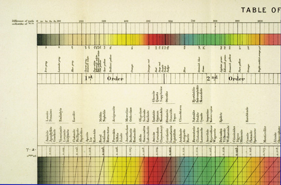
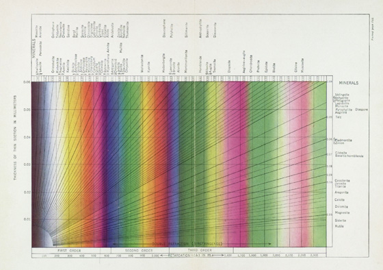
Are there differences between the interference color charts produced over the last 115 years? Which is the best? Let’s conduct a more-or-less chronological survey of Michel-Lévy interference color charts, starting with the granddaddy of them all, the original one that appeared in 1888, which we already introduced as Figure 2. This “Tableau des Biréfringences” has thickness to 60 µm, and includes four-orders of interference colors. A birefringence value of 0.040 marks the upper right corner of this chart. Mineral names are located as close as possible at their characteristic birefringence value. There are very subtle color differences in the first-order gray-white area of the chart, and it is a great help to have the descriptive name of the color. In the case of this original chart, there is a narrow strip of all four orders of interference colors along the top of the chart, together with the descriptive name of specific values of retardation. Figure 5 is a close-up of the upper-left corner of this chart that illustrates this feature. At about 24″ X 18″ in size, this is one impressive piece of work, and the opportunity to view one in person should not be missed.
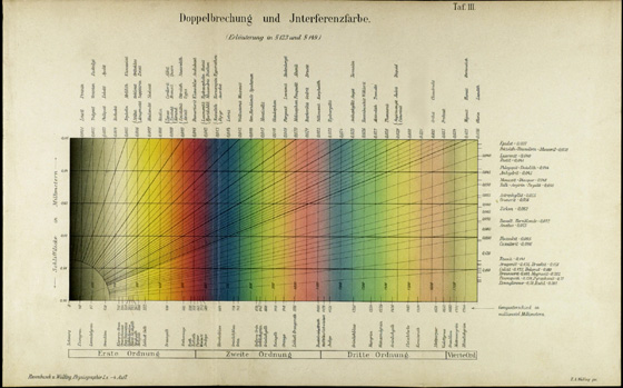
It was mentioned that the Third Edition of Rosenbusch’s famous text, Mikroskopische Physiographie, was already published when Michel-Lévy’s book came out in 1885, but by 1904 it had been expanded to a two volume, Fourth Edition (16) in collaboration with E.A. Wülfing. Volume I, called the first half, is devoted to morphology, and the principles of optical crystallography; the second volume contains the data on specific minerals. In this edition, Plate 3 (Tafel III), the Michel-Lévy chart in color is mounted at the back of Volume I; Figure 6 is an illustration of this chart. In the text (p. 283), it is referred to as “Die Michel-Lévysche Farbentafel” (The Michel-Lévy Color Table), but the actual color chart (Figure 6) is titled “Doppelbrechung und Jnterferenzfarbe” (Double Refraction and Interference Color). This chart is 15″ X 9¼”; the colored area is 10″ X 4″. This chart indicates thickness to 50 µm; three orders of interference colors, and just the start of the fourth order; the vertical lines are at 50 nm apart, with every 100 nm numbered; birefringence 0.036 is at the upper-right corner; mineral names are located at their characteristic birefringence, and the interference colors are named. This ~100 year old color chart is perfectly usable today. It is printed on card stock, and folds at two places to fit between Tables 2 and 4.
Joseph P. Iddings translated and abridged Rosenbusch’s books “for use in schools and colleges.” The Fourth Edition, published in 1900, was titled Microscopical Physiography of the Rock-Making Minerals: An Aid to the Microscopical Study of Rocks (17). Interestingly enough, although Iddings mentions Michel-Lévy in the Translator’s Preface, dated 1893, no Michel-Lévy chart appears in this book; there is only Quincke’s (8) Table of Newton’s Color Scale.
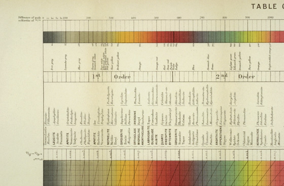
By 1906, Joseph P. Iddings published a book of his own, called Rock Minerals; Their Chemical and Physical Characters and Their Determination in Thin Section (18). He acknowledges the influence of Rosenbusch and Wülfing, but now also Michel-Lévy, and Lo and Behold, there is now an English version of Michel-Lévy’s original color chart (Figure 7); same large size (24″ X 18″); everything the same, except that all of the mineral names, names of colors, etc. have been translated into English.
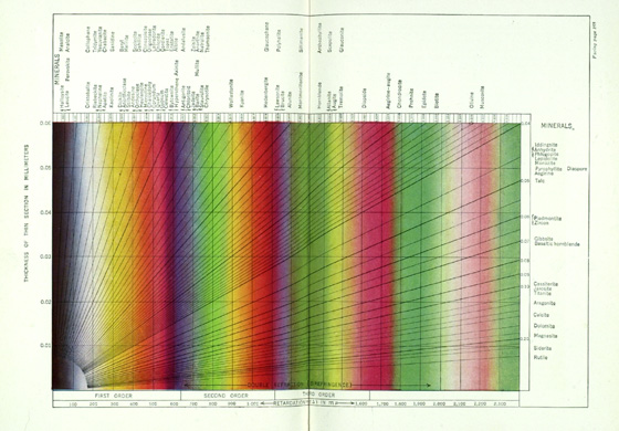
Let us stay with Iddings for the moment, because his 1906 Rock Minerals (18) went into a Second Edition in 1911 (19). The “First Thousand” copies contain the same color Michel-Lévy chart as the 1906 edition (Figure 8), but … and here is where it gets interesting … the “Second Thousand” printing (20) of the 1911 edition has a different chart (Figure 9) or, rather, an expanded version, in that the names of the minerals have been reset; more mineral names were added, and the font was changed to include use of bold letters. The printing colors in this 1911 “Second Thousand” are also more saturated than the 1906 and 1911 “First Thousand” printings. Figure 10 is a close-up of the 1911 “First Thousand” chart; Figure 11 is a close-up of the 1911 “Second Thousand” chart.
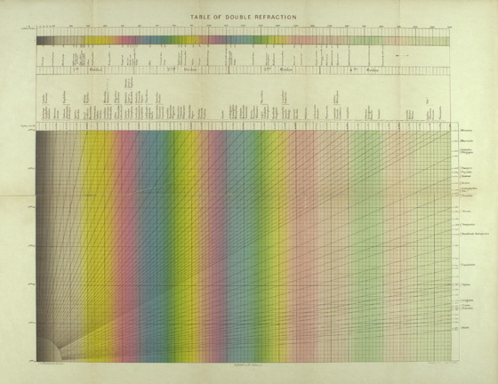
I had heard from a USGS geologist that the most accurate rendition of interference colors was attributed to the Michel-Lévy chart in the 1909 edition of Winchell and Winchell’s Elements of Optical Mineralogy (21). It turns out that the Michel-Lévy color chart (Figure 12) in this book is yet another variation of the English version of Michel-Lévy’s original. The title on this one has been changed from “Table of Birefringences” to “Table of Double Refraction,” and there are differences from the three Iddings versions in the choice of minerals included. It is the same, basic, English version of the 1888 original; that’s about a quarter-century use of the original chart and its progeny. One additional interesting feature of Winchell and Winchell’s Elements of Optical Mineralogy is a large (25″ X 18″) folded “Table of Refringence and Birefringence” (Figure 13), in which the authors plot the range of refractive indices and birefringences for a large number of minerals.


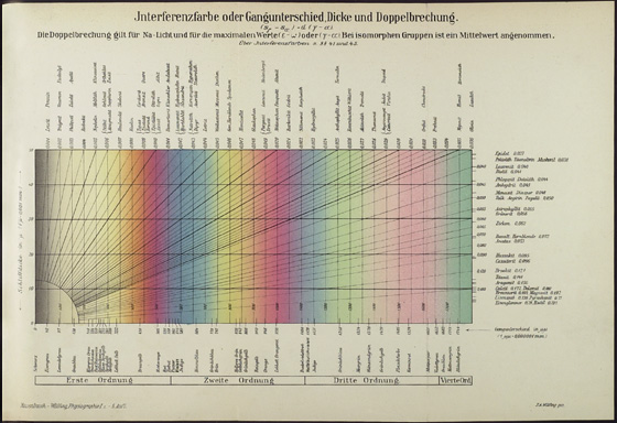
The last, great, Fifth Edition of Mikroskopische Physiographie (22) was published in the 1920s. Volume 1, Die petrographisch wichtigen Mineralien (The Petrographically Important Minerals) was published in the 1921/24 period, and Volume 2, the Spezieller Teil (the Specialized Part) that contained the mineral descriptions came out in 1927. This handsome set (Figure 14) contains a color Michel-Lévy chart (Figure 15) titled “Jnterferenzfarbe oder Gangunterschied Dicke und Doppelbrechung.” This chart is about the same as the one in the Fourth Edition (Figure 6); same size; only the title has been changed to include the influence of the thickness of the mineral, and the double refraction; the colors, however, are very different, being distinctly yellow at the far right in the Fourth Edition, and distinctly green in the Fifth Edition. This Michel-Lévy color chart from Rosenbusch and Wülfing’s Fifth Edition is the version that is said to have been framed and was on the wall of Chamot’s laboratory at Cornell University.
Over the last 75 years or so, the Michel-Lévy interference color chart appears in virtually all optical crystallography textbooks, or the chart has been supplied by the manufacturers of polarizing microscopes. Let us look at some of these.
The textbooks by Rogers and Kerr span at least four decades. The first edition of their book published in 1933 was called Thin-Section Mineralogy (1). Figure 16 illustrates the Michel-Lévy chart from the first edition, fifth impression. It is tipped in in such a way that it folds only once, in the center, and is the same size as two pages of the book (overall 11¾” X 9″). The thickness is given as “Thickness of thin section in millimeters;” the retardation is given for four orders in 100 mµ intervals (the names of the colors are not given on the chart); and common minerals are listed as close as possible to their characteristic birefringence.
Over the next seven years, the authors would learn that their text found application in other forms of mineral identification, e.g., comminuted, in addition to thin-section. Thus, the title of the 1942 second edition was changed to Optical Mineralogy (24). The interference color chart in the eighth impression of this edition is identical to the first edition; only its location within the text is different.
Rogers passed away in 1957, and in 1959 Kerr published a third edition of Optical Mineralogy (25) under his own name. The “Interference Color Chart for Common Minerals” (Figure 17), as it was now titled, is here a two-fold, tipped in at the left side; the other features remained the same.
In 1977, 44 years after the first edition, and when Kerr was already emeritus, the fourth edition of Optical Mineralogy (26) was published. The interference color chart is the same one as in the third edition 18 years earlier; now, however, it is no longer tipped in, but has been bound in, with the unfortunate consequence of losing the center portion of the chart (lost is the birefringence interval between 0.021 and 0.023) (Figure 18).
Bausch & Lomb Optical Company issued a “Michel-Lévy Scale of Birefringence” (Figure 19) which was adapted from the one in the 1942 second edition of Roger and Kerr’s Optical Mineralogy (24); the mineral names have been left off of the Bausch & Lomb version.

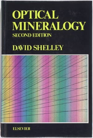
The 1985 second edition of Shelley’s book on Optical Mineralogy (27) is both memorable and striking, not so much for its interference color chart (Figure 20), as for the fact that the book’s cover has a wrap-around interference color chart (Figure 21).
Nesse’s 1991 Introduction to Optical Mineralogy (28) has an interference color chart (Figure 22) that is clearly the Zeiss issue (Figure 4); same size; two-fold, three-section, and although the names of the minerals have been left off, there is an extensive chart printed on the back of the color chart that summarizes many of the optical properties of minerals (Figure 23).
The popular 1961 text by Bloss, An Introduction to the Methods of Optical Crystallography (29), has a two-fold, three-section “Interference Color Chart for Common Minerals” based on the one in Kerr (26), but the thickness goes to 0.12 millimeters, and many more mineral names have been added. By 1999, for his Optical Crystallography (30), Bloss now has a larger, untitled, revised chart, with the minerals now showing whether they are uniaxial or biaxial, and indicating their optic sign (Figure 24).
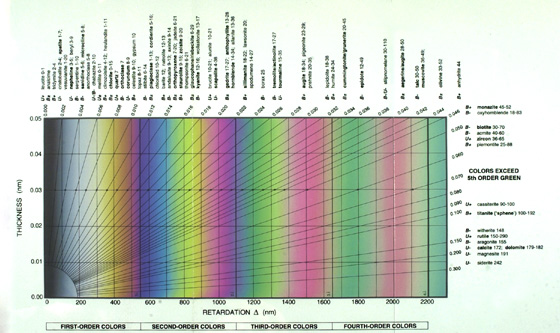
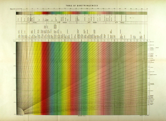
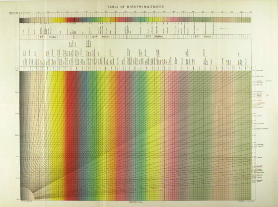
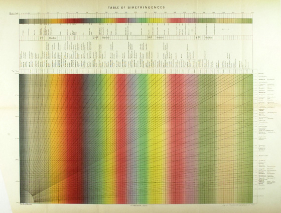
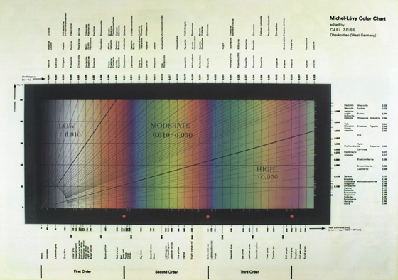
The “Michel-Lévy Birefringence Chart” used in McCrone Associates’ The Particle Atlas (31) and in the McCrone Research Institute’s Polarized Light Microscopy (32) (Figure 25) is based on the Zeiss chart (Figure 4), except that the names of the minerals are not as numerous, and now a variety of other kinds of entries appear, including natural and synthetic fibers, chemicals, food products, and drugs, better reflecting the use of the chart by analytical microscopists in industry and government, rather than by mineralogists and petrologists. Another version of the chart used for teaching purposes by the McCrone Research Institute is shown in Figure 26; this is the full Zeiss chart (Figure 4), which has been modified by indicating the birefringence qualitatively as low, moderate and high. Different texts have different ranges, but here they are low = 0–0.010, moderate = 0.010–0.050, and high = >0.050.

Almost all of the manufacturers of polarizing microscopes have, at one time or another, supplied separate interference color charts for ready reference near the polarizing microscope. Figure 27 is a vest-pocket-sized “Polarisation Colour Scale” supplied by Swift (England) over 50 years ago; it’s one of the very few charts that show the interference colors seen between parallel polarizers.

The Zeiss “Michel-Lévy Color Chart” (Figure 4) has already been described. This beautiful chart was issued as a reprint in 1963, I believe; it accompanied an article by Joseph Gahm in Zeiss’ Werkzeitschrift No. 46 (14). In this article, we learn from a footnote that the color chart was repainted by Mr. René Babillotte, and that the engravers were Meyle and Mueller, of Pforzheim, Germany [note: repainted 75 years after the original 1888 painting!].
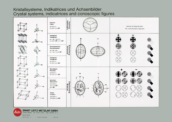
The “Polarisationsfarben/Polarization Colours” chart issued by Ernst Leitz (Figure 28) is the same large size (16½” X 11¾”) as the Zeiss chart (Figure 4), but is disposed for vertical orientation. Mineral names are located near their birefringence values, with the actual values listed for 0.048 and higher. Personally, I miss the names of the colors down in the low first order. An additional feature of this particular chart is the information on the reverse side of the chart (Figure 29); here are summaries of the crystal systems, the optical indicatrices, and conoscopic figures, with sign determination (be careful as there are a couple of errors on this side!). The chart shown here was printed in 1985. The latest edition of this Leitz chart has both the interference color chart and the summaries of the crystal systems, the optical indicatrices, and conoscopic figures, with size determination, all on one side of a poster-size wall-hanging.

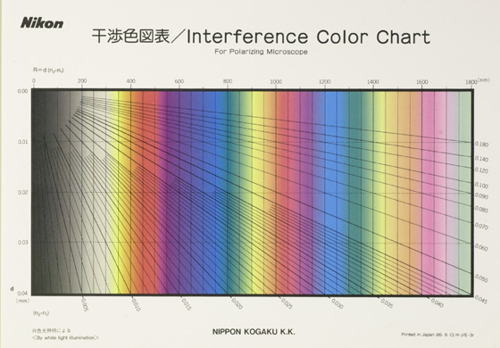
Nikon’s Interference Color Chart for Polarizing Microscope (Figure 30) appears to have been published in 1985. It is a small unfolded chart (10″ X 7″), with no names of minerals or colors. A peculiarity of this chart is its origin at the upper left; thickness goes to 40 µm. These charts were supplied by Nikon, with the purchase of a polarizing microscope.
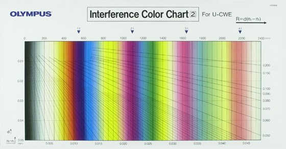
Olympus’ interference color chart (Figure 31) is not seen very often; it is intended for and supplied with the 4-order quartz wedge compensator. There are no mineral or color names; thickness goes to 50 µm; this chart, too, has its origin in the upper left corner. This two-fold, three-section chart is 13¾” X 7″.
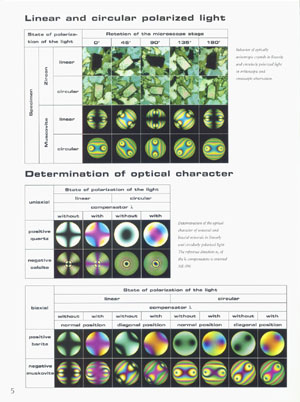
This survey has not presented all of the Michel-Lévy interference color charts, but I think I managed to hit most of the highlights. Which one is best for you? They all work–even the many black-and-white versions. I’ve always wished for a wall full of all of the interference color charts–framed! They would go well with the first-order red carpet in my study! Forty years ago, I framed the beautiful Zeiss chart (Figure 4) and had it next to my Zeiss Universal Pol microscope throughout my professional career; it has remained my favorite. This beautiful chart has again been reprinted several times over the years and the latest edition (November 2002) has been exquisitely printed. Now, however, the Michel-Lévy Color Chart is presented in a two-fold, three-section version, with addition of a diagram, in color, of the ray paths—orthoscopic and conoscopic–through a transmitted-light polarized-light microscope. There is also a page (Figure 32) devoted to linear and circular polarized light, and to the determination of optical character. The linear and circular polarized light portion illustrates the appearance of zircon and muscovite orthoscopically and conoscopically at stage rotations of 0°, 45°, 90°, 135°, and 180°. The determination of the optical character portion illustrates conoscopic views of positive and negative uniaxial crystals, and positive and negative biaxial crystals in various orientations using linear and circular polarized light, and with and without a first-order red compensator.
Today, of course, there are Michel-Lévy Birefringence charts that can be called up on the Internet via any good search engine. For the most part, these charts are posted as aids in petrographic course work, and include those from Florida State University, the University of British Columbia, and the University of Liverpool (England) – the latter includes the interference colors obtained using parallel polarizers as well.
How fortunate we polarized light microscopists are to encounter the beautiful interference colors so often in our daily work with anisotropic specimens. To be able to identify all of our unknown specimens would be doubly satisfying, and this we can do thanks to the Michel-Lévy interference color chart and its incredible ability to magically unlock the mysteries of particle identification.
References
- Les Minéraux des Roches. A. Michel-Lévy and A. Lacroix. Librairie Polytechnique, Paris (1888).
- The Particle Atlas, W.C. McCrone and J.G. Delly. 2nd Edition, Vol. 1-4 (1973), and Vol. 5 (1979) with S. Palenik. Ann Arbor Science Publishers, Ann Arbor, Michigan.
- Tableaux des Minéraux des Roches. A. Michel-Lévy and A. Lacroix. Librairie Polytechnique, Paris (1889).
- “Mémoire Sur la Double Réfraction Temporairement Produite Dans les Corps Isotropes, et Sur la Relation Entre l’Élasticité Mécanique et Entre l’Élasticité Optique.” G. Wertheim Ann. Chim. et Phys. XL, pp. 156-221. (1854).
- “Experimental – Untersuchungen. Uber Newton’sche Farbenringe u.s.w.” G. Quincke Pogg. Ann. CXXIX, pp. 177-218. (1866).
- “Uber die Farben welche in der Newton’schen Ringssystemen aufeinanderfolgen.” A. Rollet Sitzb. Adad. Wiss. Wien 77, pp. 177-261. (1878).
- “Badania Doswiad czalne Nad Skala Barw Interferencyjnch” (Études Expérimentales Sur l’Échelle des Couleurs d’Interference). C. Kraft Bull. Internat. de l’Académie des Sci. de Cracovie. sci. math. et nat., pp. 310-353. (1902).
- G. Quincke Pogg. Ann. 129, p. 177. (1866).
- Optical Crystallography 4th ed., Ernest E. Wahlstrom. John Wiley, New York (1969).
- Crystals and the Polarizing Microscope 4th ed., N.H. Hartshorne and A. Stuart. Arnold (London) (1970).
- An Introduction to the Methods of Optical Crystallography, F. Donald Bloss. Holt, Rinehart, and Winston, New York (1961).
- Manual of Petrographic Methods, Albert Johannsen. McGraw-Hill, New York (1918) [Hafner Reprint 1968].
- Mineral Optics; Principles and Techniques W.R. Phillips. W.H. Freeman (1971).
- “The Interference Color Chart According to Michel-Lévy.” Joseph Gahm. Reprint from Zeiss Werkzeitschrift No. 46, Carl Zeiss, Oberkochen, W. Germany. (1963)
- “Parallel Polarizers.” J.G. Delly. “Diffraction Lines” column in The Microscope 46 (4), pp. 207-214. (1998).
- Mikroskopische Physiographie der petrographisch wichtigen Mineralien. Two Volumes, Fourth Edition. H. Rosenbusch and E.A. Wülfing. E. Schweizerbartsche Verlagsbuchhandlung, Stuttgart (1904).
- Microscopical Physiography of the Rock-Making Minerals: An Aid to the Microscopical Study of Rocks. H. Rosenbusch. Translated and Abridged by Joseph P. Iddings. Fourth Edition, Revised. John Wiley, New York (1900).
- Rock Minerals; Their Chemical and Physical Characters and Their Determination in Thin Sections. Joseph P. Iddings. John Wiley, New York (First Edition, 1906).
- Rock Minerals; Their Chemical and Physical Characters and Their Determination in Thin Sections. Joseph P. Iddings. John Wiley, New York (Second Edition, Revised and Enlarged; First Thousand, 1911).
- Rock Minerals; Their Chemical and Physical Characters and Their Determination in Thin Sections. Joseph P. Iddings. John Wiley, New York (Second Edition, Revised and Enlarged; Second Impession with Additions; Second Thousand, 1911).
- Elements of Optical Mineralogy. N.H. Winchell and A.N. Winchell. Van Nortrand, New York (1909).
- Mikroskopische Physiographie der Mineralien und Gesteine. Two Volumes. Fifth Edition. Volume 1, Die petrographisch wichtigen Mineralien. Rosenbusch, H. and E.A. Wülfing (1921/24). Volume 2, Spezieller Teil. Rosenbusch, H. and O. Mügge (1927). Schweitzerbartsche Verlagsbuchhandlung, Stuttgart.
- Thin-Section Mineralogy. A.F. Rogers and P.F. Kerr. McGraw-Hill, New York. First Edition (1933).
- Optical Mineralogy. A.F. Rogers and P.F. Kerr. McGraw-Hill, New York. Second Edition (1942).
- Optical Mineralogy. Paul F. Kerr. McGraw-Hill, New York. Third Edition (1959).
- Optical Mineralogy. Paul F. Kerr. McGraw-Hill, New York. Fourth Edition (1977).
- Optical Mineralogy. David Shelley. Elsevier, New York. Second Edition (1985).
- Introduction to Optical Mineralogy. William Nesse. Oxford Univesity Press, New York. Second Edition (1991).
- An Introduction to the Methods of Optical Crystallography. F. Donald Bloss. Holt, New York (1961).
- Optical Crystallography. F. Donald Bloss. Mineralogical Society of America, Washington, D.C. (1999).
- The Particle Atlas. W.C. McCrone and J.G. Delly. Vol 1, Principles and Techniques. Ann Arbor Science Publishers, Ann Arbor, Michigan (1973).
- Polarized Light Microscopy. W.C. McCrone, L.B. McCrone, and J.G. Delly. McCrone Research Institute, Chicago, (numerous editions; ninth printing of revised 1977 edition, 1995).
Comments
moneer
very informative
Replies
Leslie Bolin
Thank you for your kind feedback!
Janardhana M R., Dept. of Geology, Yuvaraja's College, University of Mysore, Mysuru, India.
Great help in understanding the concept. Thank you for making known the history of development. Simple words - easy to understand. Good source of information for students.
Replies
Leslie Bolin
We're glad you found the article helpful. Thank you for reading!
add comment