Convert Foreign Currencies to USD

My name is Penny Li, a cross-border tax accountant, and I often come across instances in my work where I need to convert foreign currencies to US dollar. I have decided to build a foreign currency conversion tool in Excel that is capable of generating single-day as well as average foreign exchange rates for multiple currencies.

Objective

The objective of this tool is to automatically generate historical daily and average foreign exchange rates for 17 foreign currencies, with user inputs for the type of currency to be converted and the date or range of dates for exchange rates to be generated.

Video

Details

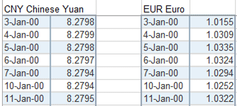
The first step is to download the exchange rates into an Excel workbook. Historical data for the exchange rates are provided by the Federal Reserve bank at this link. The data is downloaded and pasted into Excel with one set of columns per currency as illustrated below:

With the exchange rates of interest stored in Excel, we will use lookup functions to easily retrieve the desired rate for a specific time period.

In order to extract meaningful exchange rates that are useful for particular situations, we will follow the below steps to set up the conversion tool:

• List the available currency types
• Set up input cells for currency number and date
• Set up CHOOSE function with VLOOKUP to extract exchange rate on dates chosen
• Set up conversion conditions for multiplying or dividing exchange rates

List the Available Currency Types

Whether extracting exchange rates on a single date or average exchange rates over a range of dates from the stored data, it is important to have a list of all available currencies. This will be useful for referencing each foreign currency. The list below is the list that I usually use:

Set Up Input Cells for Currency Number and Date

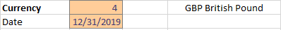
To clearly mark the input cells where the user needs to enter the currency they want to convert and the date they want the exchange rate extracted for, I have applied the Input Cell Style (Home > Cell Styles > Input) as shown below.

Set Up CHOOSE Function with VLOOKUP to Extract Exchange Rate on Dates Chosen

Below is part of the CHOOSE function used to extract the exchange rates, where C3 is the desired currency number and C4 is the desired date.

=CHOOSE(C3,VLOOKUP(C4,'FX Rate'!A:B,2,FALSE), VLOOKUP(C4,'FX Rate'!D:E,2,FALSE),...

In this formula, the CHOOSE function performs the VLOOKUP that corresponds to the currency number in C3. If the currency number is 1, then it performs a VLOOKUP on columns A:B on the FX Rate sheet. If the currency number is 2, it performs a VLOOKUP on columns D:E, and so on.

Note: For more detailed information on the functions used, check out our prior CHOOSE posts and VLOOKUP posts.

Set Up Conversion Conditions for Multiplying or Dividing Exchange Rates

Because the Euro and the British Pound are worth more than the US dollar, and the Federal reserve bank stores Australian and New Zealand dollars in values less than one, we will need to set up a short IF statement to ensure accuracy when using the exchange rates extracted.

In the IF statement set up below, the multiplication operator is to be used when the user has indicated the British Pound, Euro, NZD, or Australian dollar as the currency to be converted, while the division operator is to be used for all others.

=IF((OR(E3="GBP British Pound",E3="EUR Euro",E3="NZD New Zealand Dollar",E3="AUD Australian Dollar")),D10*C5,D10/C5)

We can then use the retrieved rate to convert the foreign currency report into a US dollar denominated report. For example, on financial statements that are as of a specific date, such as a balance sheet:

Further Variations

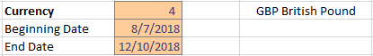
The above is only useful for converting amounts relevant to a single day to US dollar, such as for use in a balance sheet. However, this tool can be expanded to extract average exchange rates over a range of dates if we add a second date field as the end date of a period as shown below:

In order to extract the exchange rate average over a period, we will need to replace the VLOOKUP function used above with the AVERAGEIFS function, while putting the “less than or equal to” and “greater than or equal to” operators to use.

Below is the partial CHOOSE function that uses AVERAGEIFS instead of VLOOKUP, where C3 is still the currency number, C4 is the beginning date, and C5 is the ending date.

=CHOOSE(C3,AVERAGEIFS('FX Rate'!B:B,'FX Rate'!A:A,">="&C4,'FX Rate'!A:A,"<="&C5), ...

This can be useful for reports that are for a period ended, such as an income statement:

Note: for more information about the AVERAGEIFS function, check out these posts.

Use of IF Statements and Data Validation

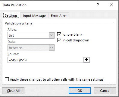
We can use the data validation feature to replace the foreign currency numbers in the above example with a drop-down menu with the currency names:

To create a data validation drop-list, head to Data > Data Validation:

Note: for more detail about Data Validation, check out these posts.

Without the currency numbers, we can use IF statements in place of the CHOOSE function, where instead of C3, we spell out the full name of the currencies.

=IF(C3="CNY Chinese Yuan",VLOOKUP(C4,'FX Rate'!A:B,2,FALSE),...

Same when determining the average exchange rate over a period:

=IF(C3="CNY Chinese Yuan",AVERAGEIFS('FX Rate'!B:B,'FX Rate'!A:A,">="&C4,'FX Rate'!A:A,"<="&C5),...

Conclusion

You can use this tool to convert foreign currency amounts to USD. I have so far used this to convert balance sheet and income statement items, but I would love to know other instances where this can be of help. Please let me know by posting a comment below … thanks!

Sample File