Lesson 3. Coordinate Reference System and Spatial Projection
This lesson covers the key spatial attributes that are needed to work with spatial data including: Coordinate Reference Systems (CRS), extent and spatial resolution.
Learning Objectives
After completing this tutorial, you will be able to:
- Describe what a Coordinate Reference System (
CRS) is - List the steps associated with plotting 2 datasets stored using different coordinate reference systems
What You Need
You will need a computer with internet access to complete this lesson and the data for week 4 of the course.
Intro to Coordinate Reference Systems
In summary - a coordinate reference system (CRS) refers to the way in which spatial data that represent the earth’s surface (which is round / 3 dimensional) are flattened so that you can “Draw” them on a 2-dimensional surface. However each using a different (sometimes) mathematical approach to performing the flattening resulting in different coordinate system grids (discussed below). These approaches to flattening the data are specifically designed to optimize the accuracy of the data in terms of length and area (more on that later too).
In this lesson you will explore what a CRS is. And how it can impact your data when you are working with it in a tool like R (or any other tool).
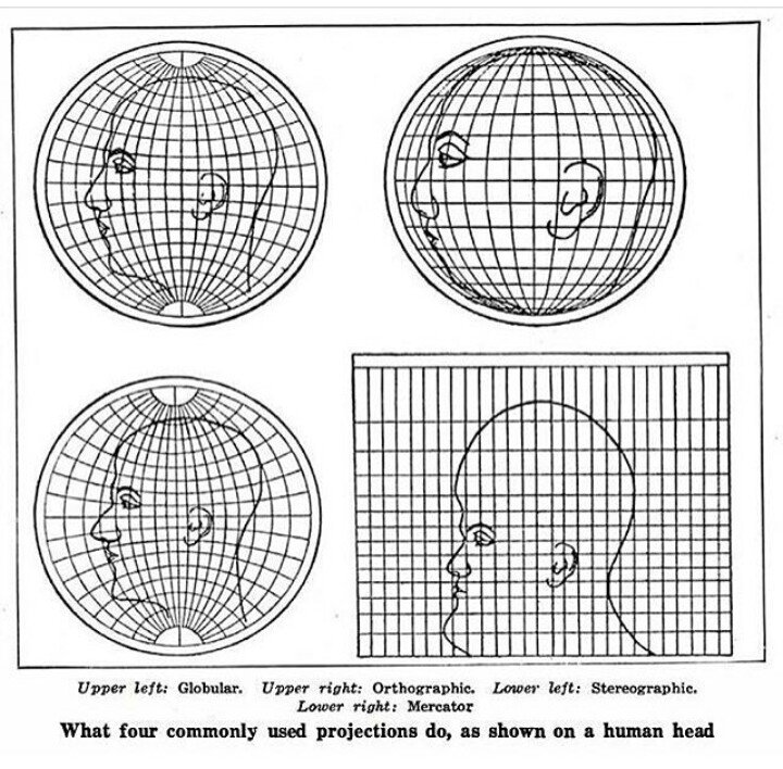
The short video below highlights how map projections can make continents look proportionally larger or smaller than they actually are.
What is a Coordinate Reference System
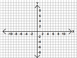
To define the location of something you often use a coordinate system. This system consists of an X and a Y value located within a 2 (or more) -dimensional space.
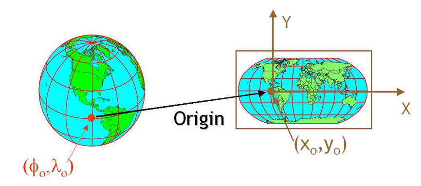
While the above coordinate system is 2-dimensional, we live on a 3-dimensional earth that happens to be “round”. To define the location of objects on the Earth, which is round, you need a coordinate system that adapts to the Earth’s shape. When you make maps on paper or on a flat computer screen, you move from a 3-Dimensional space (the globe) to a 2-Dimensional space (your computer screens or a piece of paper). The components of the CRS define how the “flattening” of data that exists in a 3-D globe space. The CRS also defines the the coordinate system itself.
A coordinate reference system (CRS) is a coordinate-based local, regional or global system used to locate geographical entities. – Wikipedia
The Components of a CRS
The coordinate reference system is made up of several key components:
- Coordinate system: The X, Y grid upon which your data is overlayed and how you define where a point is located in space.
- Horizontal and vertical units: The units used to define the grid along the x, y (and z) axis.
- Datum: A modeled version of the shape of the Earth which defines the origin used to place the coordinate system in space. You will learn this further below.
- Projection Information: The mathematical equation used to flatten objects that are on a round surface (e.g. the Earth) so you can view them on a flat surface (e.g. your computer screens or a paper map).
Why CRS is Important
It is important to understand the coordinate system that your data uses - particularly if you are working with different data stored in different coordinate systems. If you have data from the same location that are stored in different coordinate reference systems, they will not line up in any GIS or other program unless you have a program like ArcGIS or QGIS that supports projection on the fly. Even if you work in a tool that supports projection on the fly, you will want to all of your data in the same projection for performing analysis and processing tasks.
Data Tip: spatialreference.org provides an excellent online library of CRS information.
Coordinate System & Units
You can define a spatial location, such as a plot location, using an x- and a y-value - similar to your cartesian coordinate system displayed in the figure, above.
For example, the map below, generated in R with ggplot2 shows all of the continents in the world, in a Geographic Coordinate Reference System. The units are degrees and the coordinate system itself is latitude and longitude with the origin being the location where the equator meets the central meridian on the globe (0,0).
# devtools::install_github("tidyverse/ggplot2")
# load libraries
library(rgdal)
library(ggplot2)
library(rgeos)
library(raster)

#install.packages('sf')
# testing the sf package out for these lessons!
library(sf)
# set your working directory
# setwd("~/Documents/earth-analytics/")
In the plot below, you will be using the following theme. You can copy and paste this code if you’d like to use the same theme!
# turn off axis elements in ggplot for better visual comparison
newTheme <- list(theme(line = element_blank(),
      axis.text.x = element_blank(),
      axis.text.y = element_blank(),
      axis.ticks = element_blank(), # turn off ticks
      axis.title.x = element_blank(), # turn off titles
      axis.title.y = element_blank(),
      legend.position = "none")) # turn off legend
# read shapefile
worldBound <- readOGR(dsn = "data/week-04/global/ne_110m_land/ne_110m_land.shp")
# convert to dataframe
worldBound_df <- fortify(worldBound)
# plot map using ggplot
worldMap <- ggplot(worldBound_df, aes(long,lat, group = group)) +
  geom_polygon() +
  coord_equal() +
  labs(x = "Longitude (Degrees)",
       y = "Latitude (Degrees)",
      title = "Global Map - Geographic Coordinate System",
      subtitle = "WGS84 Datum, Units: Degrees - Latitude / Longitude")

worldMap

You can add three coordinate locations to your map. Note that the UNITS are in decimal degrees (latitude, longitude):
- Boulder, Colorado: 40.0274, -105.2519
- Oslo, Norway: 59.9500, 10.7500
- Mallorca, Spain: 39.6167, 2.9833
Let’s create a second map with the locations overlayed on top of the continental boundary layer.
# define locations of Boulder, CO, Mallorca, Spain and  Oslo, Norway
# store coordinates in a data.frame
loc_df <- data.frame(lon = c(-105.2519, 10.7500, 2.9833),
                lat = c(40.0274, 59.9500, 39.6167))

# add a point to the map
mapLocations <- worldMap +
                geom_point(data = loc_df,
                aes(x = lon, y = lat, group = NULL), colour = "springgreen",
                      size = 5)

mapLocations

Geographic CRS - The Good & The Less Good
Geographic coordinate systems in decimal degrees are helpful when you need to locate places on the Earth. However, latitude and longitude locations are not located using uniform measurement units. Thus, geographic CRS’s are not ideal for measuring distance. This is why other projected CRS have been developed.
Projected CRS - Robinson
You can view the same data above, in another CRS - Robinson. Robinson is a projected CRS. Notice that the country boundaries on the map - have a different shape compared to the map that you created above in the CRS: Geographic lat/long WGS84.
# reproject data from longlat to robinson CRS
worldBound_robin <- spTransform(worldBound,
                                CRS("+proj=robin"))

worldBound_df_robin <- fortify(worldBound_robin)

# force R to plot x and y values without rounding digits
# options(scipen=100)

robMap <- ggplot(worldBound_df_robin, aes(long,lat, group = group)) +
  geom_polygon() +
  labs(title = "World map (robinson)",
       x = "X Coordinates (meters)",
       y = "Y Coordinates (meters)") +
  coord_equal()

robMap

Now what happens if you try to add the same Lat / Long coordinate locations that you used above, to your map, that is using the Robinson CRS as it’s coordinate reference system?
# add a point to the map
newMap <- robMap + geom_point(data = loc_df,
                      aes(x = lon, y = lat, group = NULL),
                      colour = "springgreen",
                      size = 5)

newMap

Notice above that when you try to add lat/long coordinates in degrees to a map in a different CRS the points are not in the correct location. You need to first convert the points to the new projection - a process called reprojection. You can reproject your data using the spTransform() function in R.
Your points are stored in a data.frame which is not a spatial object. Thus, you will need to convert that data.frame to a spatial data.frame to use spTransform().
# data.frame containing locations of Boulder, CO and Oslo, Norway
loc_df
##         lon     lat
## 1 -105.2519 40.0274
## 2   10.7500 59.9500
## 3    2.9833 39.6167

# convert dataframe to spatial points data frame
loc_spdf <- SpatialPointsDataFrame(coords = loc_df, data = loc_df,
                            proj4string = crs(worldBound))

loc_spdf
## class       : SpatialPointsDataFrame
## features    : 3
## extent      : -105.2519, 10.75, 39.6167, 59.95  (xmin, xmax, ymin, ymax)
## crs         : +proj=longlat +datum=WGS84 +no_defs +ellps=WGS84 +towgs84=0,0,0
## variables   : 2
## names       :       lon,     lat
## min values  : -105.2519, 39.6167
## max values  :     10.75,   59.95
Once you have converted your data frame into a spatial data frame, you can then reproject your data.
# reproject data to Robinson
loc_spdf_rob <- spTransform(loc_spdf, CRSobj = CRS("+proj=robin"))
To make your data plot nicely with ggplot, you need to once again convert to a dataframe. You can do that by extracting the coordinates() and turning that into a data.frame using as.data.frame().
# convert the spatial object into a data frame
loc_rob_df <- as.data.frame(coordinates(loc_spdf_rob))

# turn off scientific notation
options(scipen = 10000)
# add a point to the map
newMap <- robMap + geom_point(data = loc_rob_df,
                      aes(x = lon, y = lat, group = NULL),
                      colour = "springgreen",
                      size = 5)

newMap

Compare Maps
Both of the plots above look visually different and also use a different coordinate system. Let’s look at both, side by side, with the actual graticules or latitude and longitude lines rendered on the map.
To visually see the difference in these projections as they impact parts of the world, you will use a graticules layer which contains the meridian and parallel lines.
## import graticule shapefile data
graticule <- readOGR("data/week-04/global/ne_110m_graticules_all",
                     layer = "ne_110m_graticules_15")
# convert spatial sp object into a ggplot ready, data.frame
graticule_df <- fortify(graticule)
Let’s check out your graticules. Notice they are just parallels and meridians.
# plot graticules
ggplot() +
  geom_path(data = graticule_df, aes(long, lat, group = group), linetype = "dashed", color = "grey70")

Also you will import a bounding box to make your plot look nicer!
bbox <- readOGR("data/week-04/global/ne_110m_graticules_all/ne_110m_wgs84_bounding_box.shp")
bbox_df <- fortify(bbox)

latLongMap <- ggplot(bbox_df, aes(long,lat, group = group)) +
              geom_polygon(fill = "white") +
              geom_polygon(data = worldBound_df, aes(long,lat, group = group, fill = hole)) +
              geom_path(data = graticule_df, aes(long, lat, group = group), linetype = "dashed", color = "grey70") +
  coord_equal() +  labs(title = "World Map - Geographic (long/lat degrees)")  +
  newTheme +

  scale_fill_manual(values = c("black", "white"), guide = "none") # change colors & remove legend

# add your location points to the map
latLongMap <- latLongMap +
              geom_point(data = loc_df,
                      aes(x = lon, y = lat, group = NULL),
                      colour = "springgreen",
                      size = 5)
Below, you reproject your graticules and the bounding box to the Robinson projection.
# reproject grat into robinson
graticule_robin <- spTransform(graticule, CRS("+proj=robin"))  # reproject graticule
grat_df_robin <- fortify(graticule_robin)
bbox_robin <- spTransform(bbox, CRS("+proj=robin"))  # reproject bounding box
bbox_robin_df <- fortify(bbox_robin)

# plot using robinson

finalRobMap <- ggplot(bbox_robin_df, aes(long, lat, group = group)) +
  geom_polygon(fill = "white") +
  geom_polygon(data = worldBound_df_robin, aes(long, lat, group = group, fill = hole)) +
  geom_path(data = grat_df_robin, aes(long, lat, group = group), linetype = "dashed", color = "grey70") +
  labs(title = "World Map Projected - Robinson (Meters)") +
  coord_equal() + newTheme +
  scale_fill_manual(values = c("black", "white"), guide = "none") # change colors & remove legend

# add a location layer in robinson as points to the map
finalRobMap <- finalRobMap + geom_point(data = loc_rob_df,
                      aes(x = lon, y = lat, group = NULL),
                      colour = "springgreen",
                      size = 5)
Below you plot the two maps on top of each other to make them easier to compare. To do this, you use the grid.arrange() function from the gridExtra package.
require(gridExtra)
# display side by side
grid.arrange(latLongMap, finalRobMap)

Why Multiple CRS?
You may be wondering, why bother with different CRSs if it makes your analysis more complicated? Well, each CRS is optimized to best represent the:
- shape and/or
- scale / distance and/or
- area
of features in the data. And no one CRS is great at optimizing all three elements: shape, distance AND area. Some CRSs are optimized for shape, some are optimized for distance and some are optimized for area. Some CRSs are also optimized for particular regions - for instance the United States, or Europe. Discussing CRS as it optimizes shape, distance and area is beyond the scope of this tutorial, but it’s important to understand that the CRS that you chose for your data will impact working with the data.
You will learn some of the differences between the projected UTM CRS and geographic WGS84 in the next lesson.
Optional Challenge
Compare the maps of the globe above. What do you notice about the shape of the various countries. Are there any signs of distortion in certain areas on either map? Which one is better?
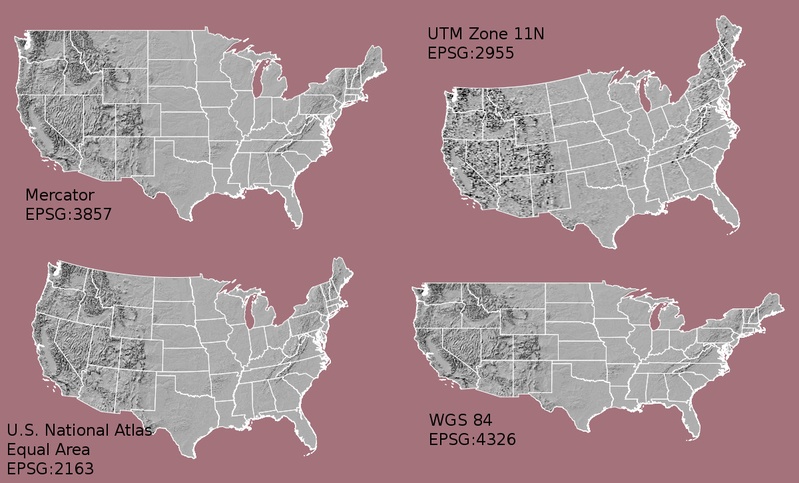
Look at the image below which depicts maps of the United States in 4 different
CRS’s. What visual differences do you notice in each map? Look up each projection online, what elements (shape,area or distance) does each projection used in the graphic below optimize?
Geographic vs. Projected CRS
The above maps provide examples of the two main types of coordinate systems:
- Geographic coordinate systems: coordinate systems that span the entire globe (e.g. latitude / longitude).
- Projected coordinate systems: coordinate systems that are localized to minimize visual distortion in a particular region (e.g. Robinson, UTM, State Plane)
You will learn these two coordinate reference systems types in more detail in the next lesson.
Additional Resources
- Read more on coordinate systems in the QGIS documentation
- For more on types of projections, visit ESRI’s ArcGIS reference on projection types.
- Read more about choosing a projection/datum
Share on
Twitter Facebook Google+ LinkedIn
Leave a Comment