Introduction

Abstract

Although the algorithms of machine-learning methods have brought issues of discrimination and fairness back to the forefront, these topics have been the subject of an extensive body of literature over the past decades. But dealing with discrimination in insurance is fundamentally an ill-defined, unsolvable problem. Nevertheless, we try to connect the dots, to explain different perspectives, going back to the legal, philosophical, and economic approaches to discrimination, before discussing the so-called concept of “actuarial fairness.” We offer some definitions, an overview of the book, as well as the datasets used in the illustrative examples throughout the chapters.

1.1 A Brief Overview on Discrimination

1.1.1 Discrimination?

Definition 1.1 (Discrimination (Merriam-Webster 2022))

Discrimination is the act, practice, or an instance of separating or distinguishing categorically rather than individually.

In this book, we use this neutral definition of “discrimination.” Nevertheless, Kroll et al. (2017) reminds us that the word “discrimination” carries a very different meaning in statistics and computer science than it does in public policy. “Among computer scientists, the word is a value-neutral synonym for differentiation or classification: a computer scientist might ask, for example, how well a facial recognition algorithm successfully discriminates between human faces and inanimate objects. But, for policymakers, “discrimination” is most often a term of art for invidious, unacceptable distinctions among people-distinctions that either are, or reasonably might be, morally or legally prohibited.” The word discrimination can then be used both in a purely descriptive sense (in the sense of making distinctions, as in this book), or in a normative manner, which implies that the differential treatment of certain groups is morally wrong, as shown by Alexander (1992), or more recently Loi and Christen (2021). To emphasize the second meaning, we can prefer the word “prejudice”, which refers to an “unjustifiable negative attitude” (Dambrum et al. (2003) and Al Ramiah et al. (2010)) or an “irrational attitude of hostility” (Merriam-Webster 2022) toward a group and its individual members.

Definition 1.2 (Prejudice (Merriam-Webster 2022))

Prejudice is (1) preconceived judgment or opinion, or an adverse opinion or leaning formed without just grounds or before sufficient knowledge; (2) an instance of such judgment or opinion; (3) an irrational attitude of hostility directed against an individual, a group, a race, or their supposed characteristics.

The definition of “discrimination” given in Correll et al. (2010) can be related to the later one “behaviour directed towards category members that is consequential for their outcomes and that is directed towards them not because of any particular deservingness or reciprocity, but simply because they happen to be members of that category.” Here, the idea of “unjustified” difference is mentioned. But what if the difference can somehow be justified? The notion of “merit” is key to the expression and experience of discrimination (we discuss this in relation to ethics later). It is not an objectively defined criterion, but one rooted in historical and current societal norms and inequalities.

Avraham (2017) explained in one short paragraph the dilemma of considering the problem of discrimination in insurance. “What is unique about insurance is that even statistical discrimination which by definition is absent of any malicious intentions, poses significant moral and legal challenges. Why? Because on the one hand, policy makers would like insurers to treat their insureds equally, without discriminating based on race, gender, age, or other characteristics, even if it makes statistical sense to discriminate (...) On the other hand, at the core of insurance business lies discrimination between risky and non-risky insureds. But riskiness often statistically correlates with the same characteristics policy makers would like to prohibit insurers from taking into account.” To illustrate this problem, and why writing about discrimination and insurance could be complicated, let us consider the example of “redlining”. Redlining has been an important issue (that we discuss further in Sect. 6.1.2), for the credit and the insurance industries, in the USA, that started in the 1930s. In 1935, the Federal Home Loan Bank Board (FHLBB) looked at more than 200 cities and created “residential security maps” to indicate the level of security for real-estate investments in each surveyed city. On the maps (see Fig. 1.1 with a collection of fictitious maps), the newest areas—those considered desirable for lending purposes—were outlined in green and known as “Type A”. “Type D” neighborhoods were outlined in red and were considered the most risky for mortgage support (on the left of Fig. 1.1). Those areas were indeed those with a high proportion of dilapidated (or dis-repaired) buildings (as we can observe on the right of Fig. 1.1). This corresponds to the first definition of “redline.”

Fig. 1.1

Map (freely) inspired by a Home Owners’ Loan Corporation map from 1937, where red is used to identify neighborhoods where investment and lending were discouraged, on the left-hand side (see Crossney 2016 and Rhynhart 2020). In the middle, some risk-related variable (a fictitious “unsanitary index”) per neighborhood of the city is presented, and on the right-hand side, a sensitive variable (the proportion of Black people in the neighborhood). Those maps are fictitious (see Charpentier et al. 2023b)

Definition 1.3 (Redline (Merriam-Webster 2022))

To redline is (1) to withhold home-loan funds or insurance from neighborhoods considered poor economic risks; (2) to discriminate against in housing or insurance.

In the 1970s, when looking at census data, sociologists noticed that red areas, where insurers did not want to offer coverage, were also those with a high proportion of Black people, and following the work of John McKnight and Andrew Gordon, “redlining” received more interest. On the map in the middle, we can observe information about the proportion of Black people. Thus, on the one hand, it could be seen as “legitimate” to have a premium for households that could reflect somehow the general conditions of houses. On the other hand, it would be discriminatory to have a premium that is a function of the ethnic origin of the policyholder. Here, the neighborhood, the “unsanitary index,” and the proportion of Black people are strongly correlated variables. Of course, there could be non-Black people living in dilapidated houses outside of the red area, Black people living in wealthy houses inside the red area, etc. If we work using aggregated data, it is difficult to disentangle information about sanitary conditions and racial information, to distinguish “legitimate” and “nonlegitimate” discrimination, as discussed in Hellman (2011). Note that within the context of “redlining,” the utilization of census and aggregated data may introduce the potential for the occurrence of an “ecological fallacy” (as discussed in King et al. (2004) or Gelman (2009)). In the 2020s, we now have much more information (so called “big data era”) and more complex models (machine-learning literature), and we will see how to disentangle this complex problem, even if dealing with discrimination in insurance is probably still an ill-defined unsolvable problem, with strong identification issues. Nevertheless, as we will see, there are many ways of looking at this problem, and we try, here, to connect the dots, to explain different perspectives.

1.1.2 Legal Perspective on Discrimination

In Kansas, more than 100 years ago, a law was passed, allowing an insurance commissioner to review rates to ensure that they were not “excessive, inadequate, or unfairly discriminatory with regards to individuals,” as mentioned in Powell (2020). Since then, the idea of “unfairly discriminatory” insurance rates has been discussed in many States in the USA (see Box 1.1).

Box 1.1 “Unfairly discriminatory” insurance rates, according to US legislation

Arkansas law (23/3/67/2/23-67-208), 1987 “A rate is not unfairly discriminatory in relation to another in the same class of business if it reflects equitably the differences in expected losses and expenses. Rates are not unfairly discriminatory because different premiums result for policyholders with like loss exposures but different expense factors, or with like expense factors but different loss exposures, if the rates reflect the differences with reasonable accuracy (...) A rate shall be deemed unfairly discriminatory as to a risk or group of risks if the application of premium discounts, credits, or surcharges among the risks does not bear a reasonable relationship to the expected loss and expense experience among the various risks.”

Maine Insurance Code (24-A, 2303), 1969 “Risks may be grouped by classifications for the establishment of rates and minimum premiums. Classification rates may be modified to produce rates for individual risks in accordance with rating plans that establish standards for measuring variations in hazards or expense provisions, or both. These standards may measure any differences among risks that may have a probable effect upon losses or expenses. No risk classification may be based upon race, creed, national origin or the religion of the insured (...) Nothing in this section shall be taken to prohibit as unreasonable or unfairly discriminatory the establishment of classifications or modifications of classifications or risks based upon size, expense, management, individual experience, purpose of insurance, location or dispersion of hazard, or any other reasonable considerations, provided such classifications and modifications apply to all risks under the same or substantially similar circumstances or conditions.”

Unfortunately, as recalled in Vandenhole (2005), there is “no universally accepted definition of discrimination,” and most legal documents usually provide (non-exhaustive) lists of the grounds on which discrimination is to be prohibited. For example, in the International Covenant on Civil and Political Rights, “the law shall prohibit any discrimination and guarantee to all persons equal and effective protection against discrimination on any ground such as race, color, sex, language, religion, political or other opinion, national or social origin, property, birth or other status” (see Joseph and Castan 2013). Such lists do not really address the question of what discrimination is. But looking for common features among those variables can be used to explain what discrimination is. For instance, discrimination is necessarily oriented toward some people based on their membership of a certain type of social group, with reference to a comparison group. Hence, our discourse should not center around the absolute assessment of how effectively an individual within a specific group is treated but rather on the comparison of the treatment that an individual receives relative to someone who could be perceived as “similar” within the reference group. Furthermore, the significance of this reference group is paramount, as discrimination does not merely entail disparate treatment, it necessitates the presence of a favored group and a disfavored group, thus characterizing a fundamentally asymmetrical dynamic. As Altman (2011), wrote, “as a reasonable first approximation, we can say that discrimination consists of acts, practices, or policies that impose a relative disadvantage on persons based on their membership in a salient social group.”

1.1.3 Discrimination from a Philosophical Perspective

As mentioned already, we should not expect to have universal rules about discrimination. For instance, Supreme Court Justice Thurgood Marshall claimed once that “a sign that says ‘men only’ looks very different on a bathroom door than on a courthouse door,” as reported in Hellman (2011). Nevertheless, philosophers have suggested definitions, starting with a distinction between “direct” and “indirect” discrimination. As mentioned in Lippert-Rasmussen (2014), it would be too simple to consider direct discrimination as intentional discrimination. A classic example would be a paternalistic employer who intends to help women by hiring them only for certain jobs, or for a promotion, as discussed in Jost et al. (2009). In that case, acts of direct discrimination can be unconscious in the sense that agents are unaware of the discriminatory motive behind decisions (related to the “implicit bias” discussed in Brownstein and Saul (2016a,b). Indirect discrimination corresponds to decisions with disproportionate effects, that might be seen as discriminatory even if that is not the objective of the decision process mechanism. A standard example could be the one where the only way to enter a public building is by a set of stairs, which could be seen as discrimination against people with disabilities who use wheelchairs, as they would be unable to enter the building; or if there were a minimum height requirement for a job where height is not relevant, which could be seen as discrimination against women, as they are generally shorter than men. On the one hand, for Young (1990), Cavanagh (2002), or Eidelson (2015), indirect discrimination should not be considered discrimination, which should be strictly limited to “intentional and explicitly formulated policies of exclusion or preference.” For Cavanagh (2002), in many cases, “it is not discrimination they object to, but its effects; and these effects can equally be brought about by other causes.” On the other hand, Rawls (1971) considered structural indirect discrimination, that is, when the rules and norms of society consistently produce disproportionately disadvantageous outcomes for the members of a certain group, relative to the other groups in society. Even if it is not intentional, it should be considered discriminatory.

Let us get back to the moral grounds, to examine why discrimination is considered wrong. According to Kahlenberg Richard (1996), racial discrimination should be considered “unfair” because it is associated with an immutable trait. Unfortunately, Boxill (1992) recalls that with such a definition, it would also be unfair to deny blind people a driver’s license. And religion challenges most definitions, as it is neither an immutable trait nor a form of disability. Another approach is to claim that discrimination is wrong because it treats persons on the basis of inaccurate generalizations and stereotypes, as suggested by Schauer (2006). For Kekes (1995), treating a person a certain way only because she is a member of a certain social group is inherently unfair, as stereotyping treats people unequally “without rational justification.” Thus, according to Flew (1993), racism is unfair because it treats individuals on the basis of traits that “are strictly superficial and properly irrelevant to all, or almost all, questions of social status and employability.” In other words, discrimination is perceived as wrong because it fails to treat individuals based on their merits. But in that case, as Cavanagh (2002) observed, “hiring on merit has more to do with efficiency than fairness,” which we will discuss further in the next section, on the economic foundations of discrimination. Finally, Lippert-Rasmussen (2006) and Arneson (1999, 2013) suggested looking at discrimination based on some consequentialist moral theory. In this approach, discrimination is wrong because it violates a rule that would be part of the social morality that maximizes overall moral value. Arneson (2013) writes that this view “can possibly defend nondiscrimination and equal opportunity norms as part of the best consequentialist public morality.”

A classical philosophical notion close to the idea of “nondiscrimination” is the concept of “equality of opportunity” (EOP). For Roemer and Trannoy (2016) “equality of opportunity” is a political ideal that is opposed to assigned-at-birth (caste) hierarchy, but not to hierarchy itself. To illustrate this point, consider the extreme case of caste hierarchy, where children acquire the social status of their parents. In contrast, “equality of opportunity” demands that the social hierarchy is determined by a form of equal competition among all members of the society. Rawls (1971) uses “equality of opportunity” to address the discrimination problem: everyone should be given a fair chance at success in a competition. This is also called “substantive equality of opportunity,” and it is often implemented through metrics such as statistical parity and equalized odds, which assume that talent and motivation are equally distributed among sub-populations. This concept can be distinguished from the “substantive equality of opportunity,” as defined in Segall (2013), where a person’s outcome should be affected only by their choices, not their circumstances.

1.1.4 From Discrimination to Fairness

Humans have an innate sense of fairness and justice, with studies showing that even 3-year-old children have demonstrated the ability to consider merit when sharing rewards, as shown by Kanngiesser and Warneken (2012), as well as chimpanzees and primates (Brosnan 2006), and many other animal species. And given that this trait is largely innate, it is difficult to define what is “fair,” although many scientists have attempted to define notions of “fair” sharing, as Brams et al. (1996) recalls. On the one hand “fair” refers to legality (and to human justice, translated into a set of laws and regulations), and in a second sense, “fair” refers to an ethical or moral concept (and to an idea of natural justice). The second reading of the word “fairness” is the most important here. According to one dictionary, fairness “consists in attributing to each person what is due to him by reference to the principles of natural justice.” And being “just” raises questions related to ethics and morality (we do not differentiate here between ethics and morality).

This has to be related to a concept introduced in Feinberg (1970), called “desert theory,” corresponding to the moral obligation that good actions must lead to better results. A student should deserve a good grade by virtue of having written a good paper, the victim of an industrial accident should deserve substantial compensation owing to the negligence of his or her employer. For Leibniz or Kant, a person is supposed to deserve happiness in virtue for being morally good. In Feinberg (1970)’s approach, “deserts” are often seen as positive, but they are also sometimes negative, like fines, dishonor, sanctions, condemnations, etc. (see Feldman (1995), Arneson (2007) or Haas (2013)). The concept of “desert” generally consists of a relationship among three elements: an agent, a deserved treatment or good, and the basis on which the agent is deserving.

We evoke in this book the “ethics of models,” or, as coined by Mittelstadt et al. (2016) or Tsamados et al. (2021), the “ethics of algorithms.” A nuance exists with respect to the “ethics of artificial intelligence,” which deals with our behavior or choices (as human beings) in relation to autonomous cars, for example, and which will attempt to answer questions such as “should a technology be adopted if it is more efficient?” The ethics of algorithms questions the choices made “by the machine” (even if they often reflect choices—or objectives—imposed by the person who programmed the algorithm), or by humans, when choices can be guided by some algorithm.

Programming an algorithm in an ethical way must be done according to a certain number of standards. Two types of norms are generally considered by philosophers. The first is related to conventions, i.e., the rules of the game (chess or Go), or the rules of the road (for autonomous cars). The second is made up of moral norms, which must be respected by everyone, and are aimed at the general interest. These norms must be universal, and therefore not favor any individual, or any group of individuals. This universality is fundamental for Singer (2011), who asks not to judge a situation with his or her own perspective, or that of a group to which one belongs, but to take a “neutral” and “fair” point of view.

As discussed previously, the ethical analyses of discrimination are related to the concept of “equality of opportunity,” which holds that the social status of individuals depends solely on the service that they can provide to society. As the second sentence of Article 1 of the 1789 Declaration of the Human Rights states, “les distinctions sociales ne peuvent être fondées que sur l’utilité commune” (translated as¹ “social distinctions may be founded only upon the general good”) or as Rawls (1971) points out, “offhand it is not clear what is meant, but we might say that those with similar abilities and skills should have similar life chances. More specifically, assuming that there is a distribution of natural assets, those who are at the same level of talent and ability, and have the same willingness to use them, should have the same prospects of success regardless of their initial place in the social system, that is, irrespective of the income class into which they are born.” In the deontological approach, inspired by Emmanuel Kant, one forgets the utilities of each person, and simply imposes norms and duties. Here, regardless of the consequences (for the community as a whole), some things are not to be done. A distinction is typically made between egalitarian and proportionalist approaches. To go further, Roemer (1996, 1998) propose a philosophical approach, whereas Fleurbaey and Maniquet (1996) and Moulin (2004) consider an economic vision. And in a more computational context, Leben (2020) goes back to normative principles to assess the fairness of a model.

All ethics courses feature thought experiments, such as the popular “streetcar dilemma.” In the original problem, stated in Foot (1967), a tram with no brakes is about to run over five people, and one of them has the opportunity to flip a switch that will cause the tram to swerve, but kill someone. What do we do? Or what should we do? Thomson (1976) suggested a different version, with a footbridge, where you can push a heavier person, who will crash into the track and die, but stop the tram. The latter version is often more disturbing because the action is indirect, and you start by murdering someone in order to save someone else. Some authors have used this thought experiment to distinguish between explanation (on scientific grounds, and based on causal arguments) and justification (based on moral precepts). This tramway experiment has been taken up in the moral psychology experiment, called, the Moral Machine project.² In this “game,” one was virtually behind the wheel of a car, and choices were proposed: “Do you run over one person or five people?”, “Do you run over an elderly person or a child?”, “Do you run over a man or a woman?” Bonnefon (2019) revisits the experiment, and the series of moral dilemmas, where they obtained more than 40 million answers, from 130 countries. Although naturally, numbers of victims were an important feature (we prefer to kill fewer people), age was also very important (priority given to young people), and legal arguments seemed to emerge (we prefer to kill pedestrians who cross outside the dedicated crossings). These questions are important for self-driving cars, as mentioned by Thornton et al. (2016).

For a philosopher, the question “How fair is this model to this group?” will always be followed by “How fair by what normative principle?” Measuring the overall effects on all those affected by the model (and not just the rights of a few) will lead to incorporating measures of fairness into an overall calculation of social costs and benefits. If we choose one approach, others will suffer. But this is the nature of moral choices, and the only responsible way to mitigate negative headlines is to develop a coherent response to these dilemmas, rather than ignore them. To speak of the ethics of models poses philosophical questions from which we cannot free ourselves, because, as we have said, a model is aimed at representing reality, “what is.” To fight against discrimination, or to invoke notions of fairness, is to talk about “what should be.” We are once again faced with the famous opposition of Hume (1739). It is a well-known property of statistical models, as well as of machine-learning ones. As Chollet (2021) wrote: “Keep in mind that machine learning can only be used to memorize patterns that are present in your training data. You can only recognize what you’ve seen before. Using machine learning trained on past data to predict the future is making the assumption that the future will behave like the past.” For when we speak of “norm,” it is important not to confuse the descriptive and the normative, or with other words, statistics (which tells us how things are) and ethics (which tells us how things should be). Statistical law is about “what is” because it has been observed to be so (e.g., humans are bigger than dogs). Human (divine, or judicial) law pertains to what is is because it has been decreed, and therefore ought to be (e.g., humans are free and equal or humans are good). One can see the “norm” as a regularity of cases, observed with the help of frequencies (or averages, as mentioned in the next chapter), for example, on the height of individuals, the length of sleep, in other words, data that make up the description of individuals. Therefore, anthropometric data have made it possible to define, for example, an average height of individuals in a given population, according to their age; in relation to this average height, a deviation of 20% more or less determines gigantism or dwarfism. If we think of road accidents, it may be considered “abnormal” to have a road accident in a given year, at an individual (micro) level, because the majority of drivers do not have an accident. However, from the insurer’s perspective (macro), the norm is that 10% of drivers have an accident. It would therefore be abnormal for no one to have an accident. This is the argument found in Durkheim (1897). From the singular act of suicide, if it is considered from the point of view of the individual who commits it, Durkheim tries to see it as a social act, therefore falling within a real norm, within a given society. From then on, suicide becomes, according to Durkheim, a “normal” phenomenon. Statistics then make it possible to quantify the tendency to commit suicide in a given society, as soon as one no longer observes the irregularity that appears in the singularity of an individual history, but a “social normality” of suicide. Abnormality is defined as “contrary to the usual order of things” (this might be considered an empirical, statistical notion), or “contrary to the right order of things” (this notion of right probably implies a normative definition), but also not conforming to the model. Defining a norm is not straightforward if we are only interested in the descriptive, empirical aspect, as actuaries do when they develop a model, but when a dimension of justice and ethics is also added, the complexity is bound to increase. We shall return in Chap. 4 to the (mathematical) properties that a “fair” or “equitable” model should be checked. Because if we ask a model to verify criteria not necessarily observed in the data, it is necessary to integrate a specific constraint into the model-learning algorithm, with a penalty related to a fairness measure (just as we use a “model complexity measure” to avoid overfit).

1.1.5 Economics Perspective on Efficient Discrimination

If jurists used the term “rational discrimination,” economists used the term “efficient” or “statistical discrimination,” such as in Phelps (1972) or Arrow (1973), following early work by Edgeworth (1922). Following Becker (1957) economists have tended to define discrimination as a situation where people who are “the same” (with respect to legitimate covariates) are treated differently. Hence, a “discrimination” corresponds here to some “disparity,” but we will frequently use the term “discrimination.” More precisely, it is necessary to distinguish two standards. One standard corresponds to “disparate treatment,” corresponding to “any economic agent who applies different rules to people in protected groups is practicing discrimination” as defined in Yinger (1998). The second discriminatory standard corresponds to “disparate impact.” This corresponds to practices that seem to be neutral, but have the effect of disadvantaging one group more than others.

Definition 1.4 (Disparate Treatment (Merriam-Webster 2022))

Disparate treatment corresponds to the treatment of an individual (as an employee or prospective juror) that is less favorable than treatment of others for discriminatory reasons (such as race, religion, national origin, sex, or disability).

Definition 1.5 (Disparate Impact (Merriam-Webster 2022))

Disparate impact corresponds to an unnecessary discriminatory effect on a protected class caused by a practice or policy (as in employment or housing) that appears to be nondiscriminatory.

In labor economics, wages should be a function of productivity, which is unobservable when signing a contract, and therefore, as discussed in Riley (1975), Kohlleppel (1983) or Quinzii and Rochet (1985), employers try to find signals. As claimed in Lippert-Rasmussen (2013), statistical discrimination occurs when “there is statistical evidence which suggests that a certain group of people differs from other groups in a certain dimension, and its members are being treated disadvantageously on the basis of this information.” Those signals are observable variables that correlate with productivity.

In the most common version of the model, employers use observable group membership as a proxy for unobservable skills, and rely on their beliefs about productivity correlates, in particular their estimates of average productivity differences between groups, as in Phelps (1972), Arrow (1973), or Bielby and Baron (1986). A variant of this theory is when there are no group differences in average productivity, but rather based on the belief that the variance in productivity is larger for some groups than for others, as in Aigner and Cain (1977) or Cornell and Welch (1996). In these cases, risk-adverse employers facing imperfect information may discriminate against groups with larger expected variances in productivity. According to England (1994), “statistical discrimination” might explain why there is still discrimination in a competitive market. For Bertrand and Duflo (2017) “statistical discrimination” is a “more disciplined explanation” than the taste-based model initiated by Becker (1957), because the former “does not involve an ad hoc (even if intuitive) addition to the utility function (animus toward certain groups) to help rationalize a puzzling behavior.”

Here, “statistical discrimination,” rather than simply providing an explanation, can lead people to see social stereotypes as useful and acceptable, and therefore help to rationalize and justify discriminatory decisions. As suggested by Tilcsik (2021), economists have theorized labor market discrimination, have constructed mathematical models that attribute discrimination to the deliberate actions of profit-maximizing firms or utility-maximizing individuals (as discussed in Charles and Guryan (2011) or Small and Pager (2020)). And this view of discrimination has influenced social science debates, legal decisions, corporate practices, and public policy discussions, as mentioned in Ashenfelter and Oaxaca (1987), Dobbin (2001), Chassonnery-Zaïgouche (2020), or Rivera (2020). The most influential economic model of discrimination is probably the “statistical discrimination theory,” discussed in the 1970s, with Phelps (1972), Arrow (1973), and Aigner and Cain (1977). Applied to labor markets, this theory claims that employers have imperfect information about the future productivity of job applicants, which leads them to use easily observable signals, such as race or gender, to infer the expected productivity of applicants, as explained in Correll and Benard (2006). Employers who practice “statistical discrimination” rely on their beliefs about group statistics to evaluate individuals (corresponding to “discrimination” as defined in Definition 1.1). In this model, discrimination does not arise from a feeling of antipathy toward members of a group, it is seen as a rational solution to an information problem. Profit-maximizing employers use all the information available to them and, as individual-specific information is limited, they use group membership as a “proxy.” Economists tend to view “statistical discrimination” as “the optimal solution to an information extraction problem” and sometimes describe it as “efficient” or “fair,” as in Autor (2003), Norman (2003) and Bertrand and Duflo (2017). It should be stressed here that this approach, initiated in the 1970s in the context of labor economics is essentially the same as the one underlying the concept of “actuarial fairness.” Observe finally that the word “statistical” used here reinforces the image of discrimination as a rational, calculated decision, even though several models do not assume that employers’ beliefs about group differences are based on statistical data, or any other type of systematic evidence. Employers’ beliefs might be based on partial or idiosyncratic observations. As mentioned in Bohren et al. (2019) it is possible to have “statistical discrimination with bad statistics” here.

1.1.6 Algorithmic Injustice and Fairness of Predictive Models

Although economists published extensively on discrimination in the job market in the 1970s, the subject has come back into the spotlight following a number of publications linked to predictive algorithms. Correctional Offender Management Profiling for Alternative Sanctions, or compas, a tool widely used as a decision aid in the US courts to assess a criminal’s chance of re-offending, based on some risk scales for general and violent recidivism, and for pretrial misconduct. After several months of investigation, Angwin et al. (2016) looked back at the output of compas in a series of articles called “Machine Bias” (and subtitled “Investigating Algorithmic Injustice”).

As pointed out (Feller et al. 2016), if we look at data from the compas dataset (from the fairness R package), in Fig. 1.2, on the one hand (on the left of the figure)

• for Black people, among those who did not re-offend, 42% were classified as high risk

  Fig. 1.2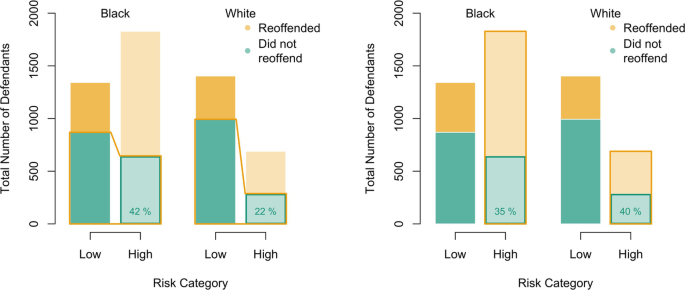

  

  Two analyses of the same descriptive statistics of compas data, with the number of defendant (1) function of the race of the defendant (Black and white), (2) the risk category, obtained from a classifier (binary, low, and high), and (3) the indicator that the defendants re-offended, or not. On the left-hand side, the analysis of Dieterich et al. (2016) and on the right-hand side, that of Feller et al. (2016)

• for white people, among those who did not re-offend, 22% were classified as high-risk

With standard terminology in classifiers and decision theory, the false-negative rate is about two times higher for Black people (42% against 22%). As Larson et al. (2016) wrote: “Black defendants were often predicted to be at a higher risk of recidivism than they actually were.” On the other hand (on the right-hand side of the figure), as Dieterich et al. (2016) observed:

• For Black people, among those who were classified as high risk, 35% did not re-offend.

• For white people, among those who were classified as high risk, 40% did not re-offend.

Therefore, as the rate of recidivism is approximately equal at each risk score level, irrespective of race, it should not be claimed that the algorithm is racist. The initial approach is called “false positive rate parity,” whereas the second one is called “predictive parity.” Obviously, there are reasonable arguments in favor of both contradictory positions. From this simple example, we see that having a valid and common definition of “fairness” or “parity” will be complicated.

Since then, many books and articles have addressed the issues highlighted in this article, namely the increasing power of these predictive decision-making tools, their ever-increasing opacity, the discrimination they replicate (or amplify), the ‘biased’ data used to train or calibrate these algorithms, and the sense of unfairness they produce. For instance, Kirkpatrick (2017) pointed out that “the algorithm itself may not be biased, but the data used by predictive policing algorithms is colored by years of biased police practices.”

And justice is not the only area where such techniques are used. In the context of predictive health systems, Obermeyer et al. (2019) observed that a widely used health risk prediction tool (predicting how sick individuals are likely to be, and the associated health care cost), that is applied to roughly 200 million individuals in the USA per year, exhibited significant racial bias. More precisely, 17.7% of patients that the algorithm assigned to receive “extra care” were Black, and if the bias in the system was corrected for, as Ledford (2019) did, the percentage should increase to 46.5%. Those “correction” techniques will be discussed in Part IV of this book, when presenting “mitigation.”

Massive data, and machine-learning techniques, have provided an opportunity to revisit a topic that has been explored by lawyers, economists, philosophers, and statisticians for the past 50 years or longer. The aim here is to revisit these ideas, to shed new light on them, with a focus on insurance, and explore possible solutions. Lawyers, in particular, have discussed these predictive models, this “actuarial justice,” as Thomas (2007), Harcourt (2011), Gautron and Dubourg (2015), or Rothschild-Elyassi et al. (2018) coined it.

The idea of bias and algorithmic discrimination is not a new one, as shown for instance by Pedreshi et al. (2008). However, over the past 20 years, the number of examples has continued to increase, with more and more interest in the media. “AI biases caused 80% of black mortgage applicants to be rejected” in Hale (2021), or “How the use of AI risks recreating the inequity of the insurance industry of the previous century” in Ito (2021). Pursuing David’s 2015 analysis, McKinsey (2017) announced that artificial intelligence would disrupt the workplace (including the insurance and banking sectors, Mundubeltz-Gendron (2019)) particularly to replace lackluster repetitive (human) work.³ These replacements raise questions, and compel the market and the regulator to be cautious. For Reijns et al. (2021), “the Dutch insurance sector makes it a mandate,” in an article on “ethical artificial intelligence,” and in France, Défenseur des droits (2020) recalls that “algorithmic biases must be able to be identified and then corrected” because “non-discrimination is not an option, but refers to a legal framework.” Bergstrom and West (2021) note that there are people writing a bill of rights for robots, or devising ways to protect humanity from super-intelligent, Terminator-like machines, but that getting into the details of algorithmic auditing is often seen as boring, but necessary.

Living with blinders on, or closing our eyes, rarely solves problems, although it has long been advocated as a solution to discrimination. As Budd et al. (2021) show, reverting to an Amazon experiment of removing names from CVs to eliminate gender discrimination does not work, because by hiding the candidate’s name, the algorithm continued to preferentially choose men over women. Why did this happen? Simply because Amazon trained the algorithm from its existing resumes, with an over-representation of men, and there are elements of a resume (apart from the name) that can reveal a person’s gender, such as a degree from a women’s university, membership of a female professional organisation, or a hobby where the sexes are disproportionately represented. Proxies that correlate more or less with the “protected” variables may sustain a form of discrimination.

In this textbook, we address these issues, limiting ourselves to actuarial models in an insurance context, and almost exclusively, the pricing of insurance contracts. In Seligman (1983), the author asks the following basic question: “If young women have fewer car accidents than young men—which is the case—why shouldn’t women get a better rate? If industry experience shows—which it does—that women spend more time in hospital, why shouldn’t women pay more?” This type of question will be the starting point in our considerations in this textbook.

Paraphrasing Georges Clémenceau,⁴ who said (in 1887) that “war is too serious a thing to be left to the military,” Worham (1985) argued that insurance segmentation was too important a task to be left to actuaries. Forty years later, we might wonder whether it is not worse to leave it to algorithms, and to clarify actuaries’ role in these debates. In the remainder, we begin by reviewing insurance segmentation and the foundations of actuarial pricing of insurance contracts. We then review the various terms mentioned in the title, namely the notion of “bias,” “discrimination,” and “fairness,” while proposing a typology of predictive models and data (in particular, the so-called “sensitive” data, which may be linked to possible discrimination).

1.1.7 Discrimination Mitigation and Affirmative Action

Mitigating discrimination is usually seen as paradoxical, because in order to avoid discrimination, we must create another discrimination. More precisely, Supreme Court Justice Harry Blackmun stated, in 1978, “in order to get beyond racism, we must first take account of race. There is no other way. And in order to treat some persons equally, we must treat them differently.” cited in Knowlton (1978), as mentioned in Lippert-Rasmussen (2020)). More formally, an argument in favor of affirmative action—called “the present-oriented anti-discrimination argument”—is simply that justice requires that we eliminate or at least mitigate (present) discrimination by the best morally permissible means of doing so, which corresponds to affirmative action. Freeman (2007) suggested a “time-neutral anti-discrimination argument,” in order to mitigate past, present, or future discrimination. But there are also arguments against affirmative action, corresponding to “the reverse discrimination objection,” as defined in Goldman (1979): some might consider that there is an absolutely ethical constraint against unfair discrimination (including affirmative action). To quote another Supreme Court Justice, in 2007, John G. Roberts of the US Supreme Court submits: “The way to stop discrimination on the basis of race is to stop discriminating on the basis of race” (Turner (2015) and Sabbagh (2007)). The arguments against affirmative action are usually based on two theoretical moral claims, according to Pojman (1998). The first denies that groups have moral status (or at least meaningful status). According to this view, individuals are only responsible for the acts they perform as specific individuals and, as a corollary, we should only compensate individuals for the harms they have specifically suffered. The second asserts that a society should distribute its goods according to merit.

1.2 From Words and Concepts to Mathematical Formalism

1.2.1 Mathematical Formalism

The starting point of any statistical or actuarial model is to suppose that observations are realizations of random variables, in some probabilistic space $(\Omega ,\mathcal {F},\mathbb {P})$ (see Rolski et al. (2009), for example, or any actuarial textbook). Therefore, let $\mathbb {P}$ denote the “true” probability measure, associated with random variables $(\boldsymbol {Z},Y)=(S,\boldsymbol {X},Y)$. Here, features $\boldsymbol {Z}$ can be split into a couple $(S,\boldsymbol {X})$, where $\boldsymbol {X}$ is the nonsensitive information whereas S is the sensitive attribute.⁵Y  is the outcome we want to model, which would correspond to the annual loss of a given insurance policy (insurance pricing), the indicator of a false claim (fraud detection), the number of visits to the dentist (partial information for insurance pricing), the occurrence of a natural catastrophe (claims management), the indicator that the policyholder will purchase insurance to a competitor (churn model), etc. Thus, here, we have a triplet $(S,\boldsymbol {X},Y)$, defined on $\mathcal {S}\times \mathcal {X}\times \mathcal {Y}$, following some unknown distribution $\mathbb {P}$. And classically, $\mathcal {D}_n=\{(\boldsymbol {z}_i,y_i)\}=\{(s_i,\boldsymbol {x}_i,y_i)\}$, where $i=1,2,\cdots ,n$, will denote a dataset, and $\mathbb {P}_n$ will denote the empirical probabilities associated with sample $\mathcal {D}_n$.

It is always assumed in this book that $\mathcal {S}$ is somehow fixed in advance, and is not learnt: gender is considered as a binary categorical variable, sensitive and protected. In most cases, s will be a categorical variable, and in order to avoid heavy notations, we simply consider a binary sensitive attribute (denoted $s\in \{{\mathtt {A}},{\mathtt {B}}\}$ to remain quite general, and avoid $\{0,1\}$ not to get confused with values taken by y in a classification problem). Recently, Hu et al. (2023b) discussed the case where $\boldsymbol {s}$ is a vector of multivariate attributes (of course possibly correlated). $\mathcal {Y}$ depends on the model considered: in a classification problem, $\mathcal {Y}$ usually corresponds to $\{0,1\}$, whereas in a regression problem, $\mathcal {Y}$ corresponds to the real line $\mathbb {R}$. We can also consider counts, when $y\in \mathbb {N}$ (i.e., $\{0,1,2,\cdots \}$). We do not discuss here the case where $\boldsymbol {y}$ is a collection of multiple predictions (also coined “multiple tasks” in the machine-learning literature, see for example Hu et al. (2023a) for applications in the context of fairness).

Throughout the book, we consider models that are formally functions $m:\mathcal {S}\times \mathcal {X}\to \mathcal {Y}$, that will be estimated from our training dataset $\mathcal {D}_n$. Considering models $m:\mathcal {X}\to \mathcal {Y}$ (sometimes coined “gender-blind” if s denotes the gender, or “color-blind” if s denotes the race, etc.) is supposed to create a more “fair” model, unfortunately, in a very weak sense (as many variables in $\boldsymbol {x}$ might be strongly correlated with s). After estimating a model, we can use it to obtain predictions, denoted $\widehat {y}$, while $m(\boldsymbol {x})$ (or $m(\boldsymbol {x},s)$) will be called the “score”, when y is a binary variable take values in $\{0,1\}$.

1.2.2 Legitimate Segmentation and Unfair Discrimination

In the previous section, we have tried to explain that there could be “legitimate” and “illegitimate” discrimination, “fair” and “unfair.” We consider here a first attempt to illustrate that issue, with a very simple dataset (with simulated data). Consider a risk, and let y denote the occurrence of that risk (hence, y is binary). As we discuss in Chap. 2, it is legitimate to ask policyholders to pay a premium that is proportional to $\mathbb {P}[Y=1]$, the probability that the risk occurs (which will be the idea of “actuarial fairness”). Assume now that this occurrence is related to a single feature x : the larger x, the more likely the risk will occur. A classic example could be the occurrence of the death of a person, where x is the age of that person. Here, the correlation between y and x is coming from a common (unobserved) factor, $x_0$. In a small dataset, toydata1 (divided into a training dataset, toydata1_train, and a validation dataset, toydata1_validation), we have simulated values, where the confounding variable $X_0$ (that will not be observed, and therefore cannot be used in the modeling process) is a Gaussian variable, $X_0\sim \mathcal {N}(0,1)$, and then

$$\displaystyle \begin{aligned} \begin{cases} X = X_0 +\epsilon,~\epsilon\sim\mathcal{N}(0,{1}/{2}^2),\\ S = \boldsymbol{1}(X_0 +\eta>0),~\eta\sim\mathcal{N}(0,{1}/{2}^2),\\ Y = \boldsymbol{1}(X_0 +\nu>0),~~\nu\sim\mathcal{N}(0,{1}/{2}^2). \end{cases}\end{aligned}$$

The sensitive attribute s, which takes values 0 (or A) and 1 (or B), does not influence y, and therefore it might not be legitimate to use it (it could be seen as an “illegitimate discrimination”). Note that $x_0$ influences all variables, x, s, and y (with a probit model for the last two), and because of that unobserved confounding variable $x_0$, all variables are here (strongly) correlated. In Fig. 1.3, we can visualize the dependence between x and y (via boxplots of x given y) on the left-hand side, and between x and s (via boxplots of x given s) on the right-hand side. For example, if $x\sim -1$, then y takes values in $\{{0},{1}\}$ respectively with 25% and 75% chance. It is a 75% and 25% chance if $x\sim +1$. Similarly, when $x\sim -1$, s is four times more likely to be in group A than in group B.

Fig. 1.3

On top, boxplot of x conditional on y, with $y\in \{{0},{1}\}$ on the left-hand side, and conditional on s, with $s\in \{{\mathtt {A}},{\mathtt {B}}\}$ on the right-hand side, from the toydata1 dataset. Below, the curve on the left-hand side is $x\mapsto \mathbb {P}[Y={1}|X=x]$ whereas the curve on the right-hand side is $x\mapsto \mathbb {P}[S={\mathtt {A}}|X=x]$. Hence, when $x=+1$, $\mathbb {P}[Y={1}|X=x]\sim {25\%}$, and therefore $\mathbb {P}[Y={0}|X=x]\sim {75\%}$ (on the left-hand side), whereas when $x=+1$, $\mathbb {P}[S={\mathtt {A}}|X=x]\sim {95\%}$, and therefore $\mathbb {P}[S={\mathtt {B}}|X=x]\sim {5\%}$ (on the right-hand side)

When fitting a logistic regression to predict y based on both x and s, from toydata1_train, observe that variable x is clearly significant, but not s (using glm in R, see Sect. 3.3 for more details about standard classifiers, starting with the logistic regression):

Coefficients:             Estimate Std. Error z value Pr(>|z|) (Intercept)  -0.2983     0.2083  -1.432    0.152 x             1.0566     0.1564   6.756 1.41e-11 ∗∗∗ s == A        0.2584     0.2804   0.922    0.357

Without the sensitive variable s, we obtain a logistic regression on x only, that could be seen as “fair through unawareness.” The estimation yields

Coefficients:             Estimate Std. Error z value Pr(>|z|) (Intercept)  -0.1390     0.1147  -1.212    0.226 x             1.1344     0.1333   8.507   <2e-16 ∗∗∗

Here, $\widehat {m}(x)$, that estimates $\mathbb {E}[Y|X=x]$, is equal to

$$\displaystyle \begin{aligned} \widehat{m}(x)=\frac{\exp[-0.1390+1.1344~x]}{1+\exp[-0.1390+1.1344~x]}. \end{aligned}$$

But it does not mean that this model is perceived as “fair” by everyone. In Fig. 1.4, we can visualize the probability that scores$\widehat {m}$ exceed a given threshold t, here $50\%$. Even without using s as a feature in the model, $\mathbb {P}[\widehat {m}(X)>t|S=s]$ does depend on s, whatever the threshold t. And if $\mathbb {E}[\widehat {m}(X)]\sim 50\%$, observe that $\mathbb {E}[\widehat {m}(X)|S={\mathtt {A}}]\sim 65\%$ while $\mathbb {E}[\widehat {m}(X)|S={\mathtt {B}}]\sim 25\%$. With our premium interpretation, it means that, on average, people that belong in group A pay a premium at least twice that paid by people in group B. Of course, ceteris paribus it is not the case, as individuals with the same x have the same prediction, whatever s, but overall, we observe a clear difference. One can easily transfer this simple example to many real-life applications.

Fig. 1.4

Distribution of the score $m( \boldsymbol {X},S)$, conditional on A and B, on the left-hand side, and distribution of the score $m( \boldsymbol {X})$ without the sensitive variable, conditional on A and B, on the right-hand side (fictitious example). In both cases, logistic regressions are considered. From this score, we can get a classifier $\widehat {y}= \boldsymbol {1}(m( \boldsymbol {z})>t)$ (where $\boldsymbol {z}$ is either $( \boldsymbol {x},s)$, on the left-hand side, or simply $\boldsymbol {x}$, on the right-hand side). Here, we consider cut-off $t=50\%$. Areas on the right of the vertical line (at $t=50\%$) correspond to the proportion of individuals classified as $\widehat {y}=1$, in both groups, A and B

Throughout this book, we provide examples of such situations, then formalize some measures of fairness, and finally discuss methods used to mitigate a possible discrimination in a predictive model $\widehat {m}$, even if $\widehat {m}$ is not a function of the sensitive attribute (fairness through unawareness).

1.3 Structure of the Book

In Part I we get back to insurance and predictive modeling. In Chap. 2, we present applications of predictive modeling in insurance, emphasizing insurance ratemaking and premium calculations, first in the context of homogeneous policyholders, and then in that of heterogeneous policyholders. We will discuss “segmentation” from a general perspective, the statistical approach being discussed in Chap. 3. In that chapter, we present standard supervised models, with general linearized models (GLMs), penalized versions, neural nets, trees, and ensemble approaches. In Chap. 4, we then address the questions of interpretation and explanation of predictive models, as well as accuracy and calibration.

In Part II, we discuss further segmentation and discrimination and sensitive attributes in the context of insurance modeling. In Chap. 5, we provide a classification and a typology of pricing variables. In Chap. 6, we discuss direct discrimination (with race, gender, age, and genetics), and indirect direction We return to biases and data, in Chap. 7, with a discussion about observations and experiments. We return to how data are collected before getting back to the popular adage “correlation is not causation,” and start to discuss causal inference and counterfactuals.

In Part III, we present various approaches to quantify fairness, with a focus in Chap. 8, on “group discrimination” concepts, whereas “individual fairness” is presented in Chap. 9.

And finally, In Part IV, we discuss the mitigation of discrimination, using three approaches: the pre-processing approach, in Chap. 10, the in-processing approach in Chap. 11, and the post-processing approach in Chap. 12.

1.4 Datasets and Case Studies

In the following chapters, and more specifically in Parts III and IV, we use both generated data and publicly available real datasets to illustrate various techniques, either to quantify a potential discrimination (in Part III) or to mitigate it (in Part IV). All the datasets are available from the GitHub repository,⁶ in R.

> library(devtools) > devtools::install_github("freakonometrics/InsurFair") > library(InsurFair)

The first toy dataset is the one discussed previously in Sect. 1.2.2, with toydata1_train and toydata1_valid, with (only) three variables y (binary outcome), s (binary sensitive attribute) and x (drawn from a Gaussian variable).

> str(toydata1_train) 'data.frame': 600 obs. of three variables:  $ x  : num  0.7939 0.5735 0.9569 0.1299 -0.0606 ...  $ s  : Factor w/ 2 levels "B","A": 1 1 2 1 2 2 2 1 1 1 ...  $ y  : Factor w/ 2 levels "0","1": 1 1 2 2 2 2 2 1 2 1 ...

As discussed, the three variables are correlated, as they are all based on an unobserved common variable z.

The toydata2 dataset consists in two generated data, $n=5000$ are used as a training sample, and $n=1000$ are used for validation. The process used to generate the data is the following:

• The binary sensitive attribute, $s\in \{{\mathtt {A}},{\mathtt {B}}\}$, is drawn, with respectively $60\%$ and $40\%$ individuals in each group

• $(x_1,x_3)\sim \mathcal {N}(\boldsymbol {\mu }_s,\boldsymbol {\varSigma }_s)$, with some correlation of $0.4$ when $s={\mathtt{A} }$ and $0.7$ when $s={\mathtt{B} }$

• $x_2\sim \mathcal {U}([0,10])$, independent of $x_1$ and $x_3$

• $\eta =\beta _0 + \beta _1 x_1 +\beta _2 x_2 + \beta _3 x_1^2+\beta _4\boldsymbol {1}_{{\mathtt{B} }}(s)$, that does not depend on $x_3$

• $y\sim \mathcal {B}(p)$, where $p=\exp (\eta )/[1+\exp (\eta )]=\mu (x_1,x_2,s)$.

In Fig. 1.5, we can visualize scatter plots with $x_1$ on the x-axis and $x_2$ on the y-axis, with on the left-hand side, colors depending on y ($y \in \{\mathtt{GOOD} , {}\mathtt{BAD} \}$, or $y\in \{\text{ {0} , {1}}\}$) and depending on s ($s\in \{\mathtt {A}~,~\mathtt {B}\}$) on the right-hand side. In Fig. 1.6, we can visualize level curves of $(x_1,x_2)\mapsto \mu (x_1,x_2,\mathtt {A})$ on the left and $(x_1,x_2)\mapsto \mu (x_1,x_2,\mathtt {B})$ on the right-hand side, where $\mu (x_1,x_2,s)$ are the true probabilities used to generate the dataset. Colors reflect the value of the probability (on the right part) and are coherent with $\{\mathtt{GOOD} , {}\mathtt{BAD} \}$.

Fig. 1.5

Scatter plot on toydata2, with $x_1$ on the x-axis and $x_2$ on the y-axis, with on the left-hand side, colors depending on the outcome y ($y\in \{\mathtt{GOOD} , {}\mathtt{BAD} \}$, or $y\in \{\text{ {0} , {1}}\}$) and depending on the sensitive attribute s ($s\in \{\mathtt {A}~,~\mathtt {B}\}$) on the right-hand side

Fig. 1.6

Level curves of $(x_1,x_2)\mapsto \mu (x_1,x_2,\mathtt {A})$ on the left-hand side and $(x_1,x_2)\mapsto \mu (x_1,x_2,\mathtt {B})$ on the right-hand side, the true probabilities used to generate the toydata2 dataset. The blue area in the lower-left corner corresponds to $\widehat {y}$ close to ${0}\,\,( \mbox{blue})$ (or GOOD (blue) risk), whereas the red area in the upper right corner corresponds to $\widehat {y}$ close to ${1}\,\,( \mbox{red})$ (or BAD (red) risk)

Then, there will be real data. The GermanCredit dataset, collected in Hofmann (1990) and used in the CASdataset package, from Charpentier (2014), contains 1000 observations and 23 attributes. The variable of interest y is a binary variable indicating whether a person experienced a default of payment. There are $70\%$ of 0’s (“good” risks), $30\%$ of 1’s (“bad” risks). The sensitive attribute is the gender of the person (binary, with 69% women (B) and 31% men (A), but we can also use the age, treated as categorical.

The FrenchMotor datasets, from Charpentier (2014), are in personal motor insurance, with underwriting data, and information about claim occurrence (here considered as binary). It is obtained as the aggregation of freMPL1, freMPL2, freMPL3 and freMPL4 from the CASdataset R package, while keeping only observations with exposure exceeding $90\%$. Here, the sensitive attribute is $s=\mathtt {Gender}$, which is a binary feature, and the goal is to create a score that reflects the probability of claiming a loss (during the year). The entire dataset contains $n=12{,}437$ policyholders and 18 variables. A subset with 70% of the observations is used for training, and 30% are used for observation. Note that variable SocioCateg contains here nine categories (only the first digit in the categories is considered). In numerical applications, two specific individuals (named Andrew and Barbara) are considered, to illustrate various points.

The telematic dataset is an original dataset, containing 1177 insurance contracts, observed over 2 years. We have claims data for 2019 (here claim is binary, no or yes, 13% of the policyholders claimed a loss), the age (age) and the gender (gender) of the driver, as well as some telematic data for 2018 (including Total_Distance, Total_Time, as well as Drive_Score, Style_Score, Corner_Score, Acceleration_Score or Braking_Score, in addition to some binary scores related to “heavy” acceleration or braking).

References

Aigner DJ, Cain GG (1977) Statistical theories of discrimination in labor markets. Ind Labor Relat Rev 30(2):175–187
Al Ramiah A, Hewstone M, Dovidio JF, Penner LA (2010) The social psychology of discrimination: Theory, measurement and consequences. In: Making equality count, pp 84–112. The Liffey Press, Dublin
Alexander L (1992) What makes wrongful discrimination wrong? biases, preferences, stereotypes, and proxies. Univ Pennsylvania Law Rev 141(1):149–219
Altman A (2011) Discrimination. Stanford Encyclopedia of Philosophy
Angwin J, Larson J, Mattu S, Kirchner L (2016) Machine bias: There’s software used across the country to predict future criminals and it’s biased against blacks. ProPublica May 23
Arneson RJ (1999) Egalitarianism and responsibility. J Ethics 3:225–247
Arneson RJ (2007) Desert and equality. In: Egalitarianism: New essays on the nature and value of equality, pp 262–293. Oxford University Press, Oxford
Arneson RJ (2013) Discrimination, disparate impact, and theories of justice. In: Hellman D, Moreau S (eds) Philosophical foundations of discrimination law, vol 87, p 105. Oxford University Press, Oxford
Arrow KJ (1973) The theory of discrimination. In: Ashenfelter O, Rees A (eds) Discrimination in labor markets. Princeton University Press, Princeton
Ashenfelter O, Oaxaca R (1987) The economics of discrimination: Economists enter the courtroom. Am Econ Rev 77(2):321–325
Autor D (2003) Lecture note: the economics of discrimination-theory. Graduate Labor Economics, Massachusetts Institute of Technology, pp 1–18
Avraham R (2017) Discrimination and insurance. In: Lippert-Rasmussen K (ed) Handbook of the Ethics of Discrimination, Routledge, pp 335–347
Becker GS (1957) The economics of discrimination. University of Chicago Press, Chicago
Bergstrom CT, West JD (2021) Calling bullshit: the art of skepticism in a data-driven world. Random House Trade Paperbacks
Bertrand M, Duflo E (2017) Field experiments on discrimination. Handbook Econ Field Exp 1:309–393
Bielby WT, Baron JN (1986) Men and women at work: Sex segregation and statistical discrimination. Am J Sociol 91(4):759–799
Bohren JA, Haggag K, Imas A, Pope DG (2019) Inaccurate statistical discrimination: An identification problem. Tech. rep., National Bureau of Economic Research
Bonnefon JF (2019) La voiture qui en savait trop. L’intelligence artificielle a-t-elle une morale? Humensciences Editions
Boxill BR (1992) Blacks and social justice. Rowman & Littlefield, Lanham
Brams SJ, Brams SJ, Taylor AD (1996) Fair division: from cake-cutting to dispute resolution. Cambridge University Press, Cambridge
Brosnan SF (2006) Nonhuman species’ reactions to inequity and their implications for fairness. Social Justice Res 19(2):153–185
Brownstein M, Saul J (2016a) Implicit bias and philosophy, volume 1: Metaphysics and epistemology. Oxford University Press, Oxford
Brownstein M, Saul J (2016b) Implicit bias and philosophy, volume 2: Moral responsibility, structural injustice, and ethics. Oxford University Press, Oxford
Budd LP, Moorthi RA, Botha H, Wicks AC, Mead J (2021) Automated hiring at Amazon. Universiteit van Amsterdam E-0470
Cavanagh M (2002) Against equality of opportunity. Clarendon Press, Oxford, England
Charles KK, Guryan J (2011) Studying discrimination: Fundamental challenges and recent progress. Annu Rev Econ 3(1):479–511
Charpentier A (2014) Computational actuarial science with R. CRC Press, Boca Raton
Charpentier A, Hu F, Ratz P (2023b) Mitigating discrimination in insurance with Wasserstein barycenters. BIAS, 3rd Workshop on Bias and Fairness in AI, International Workshop of ECML PKDD
Chassonnery-Zaïgouche C (2020) How economists entered the ‘numbers game’: Measuring discrimination in the us courtrooms, 1971–1989. J Hist Econ Thought 42(2):229–259
Chollet F (2021) Deep learning with Python. Simon and Schuster, New York
Cornell B, Welch I (1996) Culture, information, and screening discrimination. J Polit Econ 104(3):542–571
Correll J, Judd CM, Park B, Wittenbrink B (2010) Measuring prejudice, stereotypes and discrimination. The SAGE handbook of prejudice, stereotyping and discrimination, pp 45–62
Correll SJ, Benard S (2006) Biased estimators? comparing status and statistical theories of gender discrimination. In: Advances in group processes, vol 23, pp 89–116. Emerald Group Publishing Limited, Leeds, England
Crossney KB (2016) Redlining. https://philadelphiaencyclopediaorg/essays/redlining/
Dambrum M, Despres G, Guimond S (2003) On the multifaceted nature of prejudice: Psychophysiological responses to ingroup and outgroup ethnic stimuli. Current Res Soc Psychol 8(14):187–206
David H (2015) Why are there still so many jobs? The history and future of workplace automation. J Econ Perspect 29(3):3–30
Défenseur des droits (2020) Algorithmes: prévenir l’automatisation des discriminations. https://www.defenseurdesdroits.fr/sites/default/files/2023-07/ddd_rapport_algorithmes_2020_EN_20200531.pdf
Dieterich W, Mendoza C, Brennan T (2016) Compas risk scales: Demonstrating accuracy equity and predictive parity. Northpointe Inc 7(7.4):1
Dobbin F (2001) Do the social sciences shape corporate anti-discrimination practice: The United States and France. Comparative Labor Law Pol J 23:829
Durkheim É (1897) Le suicide: étude sociologique. Félix Alcan Editeur
Edgeworth FY (1922) Equal pay to men and women for equal work. Econ J 32(128):431–457
Eidelson B (2015) Discrimination and disrespect. Oxford University Press, Oxford
England P (1994) Neoclassical economists’ theories of discrimination. In: Equal employment opportunity: Labor market discrimination and public policy, Aldine de Gruyter, pp 59–70
Feinberg J (1970) Justice and personal desert. In: Feinberg J (ed) Doing and deserving. Princeton University Press, Princeton
Feldman F (1995) Desert: Reconsideration of some received wisdom. Mind 104(413):63–77
Feller A, Pierson E, Corbett-Davies S, Goel S (2016) A computer program used for bail and sentencing decisions was labeled biased against blacks. it’s actually not that clear. The Washington Post October 17
Fleurbaey M, Maniquet F (1996) A theory of fairness and social welfare. Cambridge University Press, Cambridge
Flew A (1993) Three concepts of racism. Int Soc Sci Rev 68(3):99
Foot P (1967) The problem of abortion and the doctrine of the double effect. Oxford Rev 5
Freeman S (2007) Rawls. Routledge
Gautron V, Dubourg É (2015) La rationalisation des outils et méthodes d’évaluation: de l’approche clinique au jugement actuariel. Criminocorpus Revue d’Histoire de la justice, des crimes et des peines
Gelman A (2009) Red state, blue state, rich state, poor state: Why Americans vote the way they do. Princeton University Press, Princeton
Goldman A (1979) Justice and reverse discrimination. Princeton University Press, Princeton
Haas D (2013) Merit, fit, and basic desert. Philos Explorat 16(2):226–239
Hale K (2021) A.i. bias caused 80% of black mortgage applicants to be denied. Forbes 09/2021
Harcourt BE (2011) Surveiller et punir à l’âge actuariel. Déviance et Société 35:163
Hellman D (2011) When is discrimination wrong? Harvard University Press, Harvard
Hofmann HJ (1990) Die anwendung des cart-verfahrens zur statistischen bonitätsanalyse von konsumentenkrediten. Zeitschrift fur Betriebswirtschaft 60:941–962
Hu F, Ratz P, Charpentier A (2023a) Fairness in multi-task learning via Wasserstein barycenters. Joint European Conference on Machine Learning and Knowledge Discovery in Databases – ECML PKDD
Hu F, Ratz P, Charpentier A (2023b) A sequentially fair mechanism for multiple sensitive attributes. ArXiv 2309.06627
Hume D (1739) A treatise of human nature. Cambridge University Press, Cambridge
Ito J (2021) Supposedly ‘fair’ algorithms can perpetuate discrimination. Wired 02.05.2019
Joseph S, Castan M (2013) The international covenant on civil and political rights: cases, materials, and commentary. Oxford University Press, Oxford
Jost JT, Rudman LA, Blair IV, Carney DR, Dasgupta N, Glaser J, Hardin CD (2009) The existence of implicit bias is beyond reasonable doubt: A refutation of ideological and methodological objections and executive summary of ten studies that no manager should ignore. Res Organizat Behav 29:39–69
Kahlenberg Richard D (1996) The remedy. class, race and affirmative action. Basic, New York
Kanngiesser P, Warneken F (2012) Young children consider merit when sharing resources with others. PLOS ONE 8(8):e43979
Kekes J (1995) The injustice of affirmative action involving preferential treatment. In: Cahn S (ed) The Affirmative Action Debate, Routledge, pp 293–304
King G, Tanner MA, Rosen O (2004) Ecological inference: New methodological strategies. Cambridge University Press, Cambridge
Kirkpatrick K (2017) It’s not the algorithm, it’s the data. Commun ACM 60(2):21–23
Knowlton RE (1978) Regents of the University of California v. Bakke. Arkansas Law Rev 32:499
Kohlleppel L (1983) Multidimensional market signalling. Institut für Gesellschafts und Wirtschaftswissenschaften, Wirtschaftstheoretische Abteilung
Kroll JA, Huey J, Barocas S, Felten EW, Reidenberg JR, Robinson DG, Yu H (2017) Accountable algorithms. Univ Pennsylvania Law Rev 165:633–705
Larson J, Mattu S, Kirchner L, Angwin J (2016) How we analyzed the compas recidivism algorithm. ProPublica 23-05
Leben D (2020) Normative principles for evaluating fairness in machine learning. In: Proceedings of the AAAI/ACM Conference on AI, Ethics, and Society, pp 86–92
Ledford H (2019) Millions affected by racial bias in health-care algorithm. Nature 574(31):2
Lippert-Rasmussen K (2006) The badness of discrimination. Ethical Theory Moral Pract 9:167–185
Lippert-Rasmussen K (2013) Discrimination. In: LaFollette H (ed) The international encyclopedia of ethics. Wiley-Blackwell, New York
Lippert-Rasmussen K (2014) Born free and equal? A philosophical inquiry into the nature of discrimination. Oxford University Press, Oxford
Lippert-Rasmussen K (2020) Making sense of affirmative action. Oxford University Press, Oxford
Loi M, Christen M (2021) Choosing how to discriminate: navigating ethical trade-offs in fair algorithmic design for the insurance sector. Philos Technol, 1–26
McKinsey (2017) Technology, jobs and the future of work. McKinsey Global Institute
Merriam-Webster (2022) Dictionary. Merriam-Webster
Mittelstadt BD, Allo P, Taddeo M, Wachter S, Floridi L (2016) The ethics of algorithms: Mapping the debate. Big Data Soc 3(2):2053951716679679
Moulin H (2004) Fair division and collective welfare. MIT Press, Cambridge, MA
Mundubeltz-Gendron S (2019) Comment l’intelligence artificielle va bouleverser le monde du travail dans l’assurance. L’Argus de l’Assurance 10/04
Norman P (2003) Statistical discrimination and efficiency. Rev Econ Stud 70(3):615–627
Obermeyer Z, Powers B, Vogeli C, Mullainathan S (2019) Dissecting racial bias in an algorithm used to manage the health of populations. Science 366(6464):447–453
Pedreshi D, Ruggieri S, Turini F (2008) Discrimination-aware data mining. In: Proceedings of the 14th ACM SIGKDD International Conference on Knowledge Discovery and Data Mining, KDD ’08, pp 560–568. Association for Computing Machinery
Phelps ES (1972) The statistical theory of racism and sexism. Am Econ Rev 62(4):659–661
Pojman LP (1998) The case against affirmative action. Int J Appl Philos 12(1):97–115
Powell L (2020) Risk-based pricing of property and liability insurance. J Insurance Regulat 1:1–23
Quinzii M, Rochet JC (1985) Multidimensional signalling. J Math Econ 14(3):261–284
Rawls J (1971) A theory of justice: Revised edition. Harvard University Press, Harvard
Reijns T, Weurding R, Schaffers J (2021) Ethical artificial intelligence – the dutch insurance industry makes it a mandate. KPMG Insights 03/2021
Rhynhart R (2020) Mapping the legacy of structural racism in Philadelphia. Office of the Controller, Philadelphia
Riley JG (1975) Competitive signalling. J Econ Theory 10(2):174–186
Rivera LA (2020) Employer decision making. Annu Rev Sociol 46:215–232
Roemer JE (1996) Theories of distributive justice. Harvard University Press, Harvard
Roemer JE (1998) Equality of opportunity. Harvard University Press, Harvard
Roemer JE, Trannoy A (2016) Equality of opportunity: Theory and measurement. J Econ Literature 54(4):1288–1332
Rolski T, Schmidli H, Schmidt V, Teugels JL (2009) Stochastic processes for insurance and finance. Wiley, New York
Rothschild-Elyassi G, Koehler J, Simon J (2018) Actuarial justice, chap 14, pp 194–206. Wiley, New York
Sabbagh D (2007) Equality and transparency: A strategic perspective on affirmative action in American law. Springer, New York
Schauer F (2006) Profiles, probabilities, and stereotypes. Harvard University Press, Harvard
Segall S (2013) Equality and opportunity. Oxford University Press, Oxford
Seligman D (1983) Insurance and the price of sex. Fortune February 21st
Singer P (2011) Practical ethics. Cambridge University Press, Cambridge
Small ML, Pager D (2020) Sociological perspectives on racial discrimination. J Econ Perspect 34(2):49–67
Thomas RG (2007) Some novel perspectives on risk classification. Geneva Papers Risk Insurance Issues Pract 32(1):105–132
Thomson JJ (1976) Killing, letting die, and the trolley problem. Monist 59(2):204–217
Thornton SM, Pan S, Erlien SM, Gerdes JC (2016) Incorporating ethical considerations into automated vehicle control. IEEE Trans Intell Transp Syst 18(6):1429–1439
Tilcsik A (2021) Statistical discrimination and the rationalization of stereotypes. Am Sociol Rev 86(1):93–122
Tsamados A, Aggarwal N, Cowls J, Morley J, Roberts H, Taddeo M, Floridi L (2021) The ethics of algorithms: key problems and solutions, pp 1–16. AI & Society
Turner R (2015) The way to stop discrimination on the basis of race. Stanford J Civil Rights Civil Liberties 11:45
Vandenhole W (2005) Non-discrimination and equality in the view of the UN human rights treaty bodies. Intersentia nv
Worham L (1985) Insurance classification: too important to be left to the actuaries. Univ Michigan J Law 19:349
Yinger J (1998) Evidence on discrimination in consumer markets. J Econ Perspect 12(2):23–40
Young IM (1990) Justice and the politics of difference. Princeton University Press, Princeton
Author information
Authors and Affiliations
Rights and permissions
Copyright information
© 2024 The Author(s), under exclusive license to Springer Nature Switzerland AG
About this chapter
Cite this chapter
Charpentier, A. (2024). Introduction. In: Insurance, Biases, Discrimination and Fairness. Springer Actuarial. Springer, Cham. https://doi.org/10.1007/978-3-031-49783-4_1
Download citation
DOI: https://doi.org/10.1007/978-3-031-49783-4_1
Published:
Publisher Name: Springer, Cham
Print ISBN: 978-3-031-49782-7
Online ISBN: 978-3-031-49783-4
eBook Packages: Mathematics and StatisticsMathematics and Statistics (R0)