Hands-on Tutorials, 3D Python
3D Point Cloud Clustering Tutorial with K-means and Python
A complete hands-on python guide for creating 3D semantic segmentation datasets. Learn how to transform unlabelled point cloud data through unsupervised segmentation with K-Means clustering.

If you are on the quest for a (Supervised) Deep Learning algorithm for semantic segmentation — keywords alert 😁 — you certainly have found yourself searching for some high-quality labels + a high quantity of data points.
In our 3D data world, the unlabelled nature of the 3D point clouds makes it particularly challenging to answer both criteria: without any good training set, it is hard to “train” any predictive model.
Should we explore python tricks and add them to our quiver to quickly produce awesome 3D labeled point cloud datasets?
Let us dive right in! 🤿
Foreword on clustering for unsupervised workflows
Why unsupervised segmentation & clustering is the “bulk of AI”?
Deep Learning (DL) through supervised systems is extremely useful. DL architectures have profoundly changed the technological landscape in the last years. However, if we want to create brilliant machines, Deep learning will need a qualitative renewal — rejecting the notion that bigger is better. Several approaches exist today to achieve this milestone, and on top of it all, unsupervised or self-supervised directions are game-changers.

Clustering algorithms are often used for exploratory data analysis. They also constitute the bulk of the processes in AI classification pipelines to create nicely labeled datasets in an unsupervised/self-learning fashion.
This sentence extracted from the previous article, “Fundamentals to clustering high-dimensional data” summarizes our driver to quickly explore a hands-on way to create your semi-automated labeling pipeline. Exciting! But of course, if you feel like you need some quick refreshers on the theory, you can find the full explanation in the article below.
How to define Clustering?
In one sentence, clustering means grouping similar items or data points together. K-means is a specific algorithm to compute such a clustering.
So what are those data points that we may want to cluster? These can be arbitrary points, such as 3D points recorded with a LiDAR scanner.

But they can also represent spatial coordinates, color values in your dataset (image, point cloud, …), or other features such as keypoint descriptors extracted from an image to build a bag of words dictionary.


You can see them as arbitrary vectors in space, each holding a set of attributes. Then, we gather many of those vectors in a defined “feature space”, and we want to represent them with a small number of representatives. But the big question here is, what should those representatives look like?
K-Means Clustering
K-Means is a very simple and popular algorithm to compute such a clustering. It is typically an unsupervised process, so we do not need any labels, such as in classification problems.
The only thing we need to know is a distance function. A function that tells us how far two data points are apart from each other. In the simplest form, this is the Euclidean distance. But depending on your application, you may also want to select a different distance function. Then, we can decide if two data points are similar to one another, thus if they belong to the same cluster.
How does K-Means work?
It represents all the data points with K representatives, which gave the algorithm its name. So K is a user-defined number that we put into the system. For example, take all the data points and represent them with three points in space.

So in the example above, the blue points are the input data points, and we set K=3. That means we want to represent those data points with three different representatives. Then those representatives illustrated by the colored red points orient the corresponding assignments of data points to the “best” representatives. We then obtain three clusters of points, green, purple, and yellow.
And K-means does it in a way that minimizes the squared distance between the data point and its closest representative. The algorithmic part that achieves this is constructed in two simple steps iteratively remade: the initialization and the assignment:
- We randomly initialize K centroids points as representatives, and we compute a data association of every data point to the closest centroid. So it is a nearest neighbor query that we are doing here.
- Every data point gets assigned to its closest centroid, and then we reconfigure the location of each centroid in our space. It is done by computing the primary vector out of all the data points assigned to that centroid, which changes its location.
So in the next iteration of the algorithm, we will get a new assignment and then a new centroid location, and we repeat this process until convergence.

💡Hint: We should note that K-Means is not an optimal algorithm. This means that K-Means tries to minimize the distance function, but we are not guaranteed to find a global minimum. So depending on your starting location, you may end up with a different result for your K-Means clustering. Suppose we want to implement K-Means in a fast manner. In that case, we typically need to have an approximate nearest neighbor function in our space because this is the most time-consuming operation done with this algorithm. Good news, I will hint k-means++ later on 😉.
K-Means is thus a relatively simple two-step iterative approach to finding representatives for a potentially large number of data points in high dimensional spaces. Now that the theory is over let us dive into a fun python code implementation in five steps🤲!
1. The Point Cloud Workflow definition
Aerial LiDAR Point Cloud Dataset
The first step of our hands-on tutorial is to gather a nice dataset! This time, I want to share another excellent place to find cool LiDAR datasets: the Geoservices of the National Geography Institute of France. The LiDAR HD campaign of the IGN in France starts an OpenData gathering where you can get crisp 3D point clouds of some regions of France!
I went on the portal above, selected one tile, extracted a sub-tile from it, deleted the georeferencing information, prepared some extra attributes part of a LiDAR file, and then made it available in my Open Data Drive Folder. The data you are interested in are KME_planes.xyz and KME_cars.xyz. You can jump at the Flyvast WebGL extract if you want to visualize them online.
The overall loop strategy
I propose to follow a simple procedure that you can replicate to label your point cloud datasets, as illustrated below quickly.

🤓 Note: The strategy is a little extract from one of the documents given on the online courses that I host at the 3D Geodata Academy. This tutorial will cover steps 7 to 10, the other ones covered in depth in the course, or by following the coding guide below.
2. Setting up our 3D python context
In this hands-on point cloud tutorial, I focused on efficient and minimal library usage. We could do all with other libraries like open3d, pptk, pytorch3D … But for the sake of mastering python, we will do it all with NumPy, Matplotlib, and ScikitLearn. Six lines of code to start your script:
import numpy as np
import matplotlib.pyplot as plt
from mpl_toolkits import mplot3d
from sklearn.cluster import KMeans
from sklearn.cluster import DBSCAN
Nice, from there, I propose that we relatively express our paths, separating the data_folder containing our datasets from the dataset name to switch easily on the fly:
data_folder=”../DATA/”
dataset=”KME_planes.xyz”
From there, I want to illustrate a nice trick to load your point cloud with Numpy. The intuitive way would be to load everything in a pcd point cloud variable, such as pcd=np.loadtxt(data_folder+dataset). But because we will play a bit with the features, let us save some time by unpacking on the fly each column in a variable. How cool is Numpy? 😆
x,y,z,illuminance,reflectance,intensity,nb_of_returns = np.loadtxt(data_folder+dataset,skiprows=1, delimiter=’;’, unpack=True)Nice! We now have everything to play around with! Because of the essence of K-Means, we have to be careful with the ground element omnipresence, which would provide something weird like the below:


To avoid weird results, we should handle what we consider outliers, the ground. Below is a direct trick for this, without injecting too much-constraining knowledge.
3. Point Cloud quick selection
Let me illustrate how to handle this with a tiny supervision step through Matplotlib. It also allows me to give you pieces of code that always come in handy with subplot creation and line layering. We will check on a 2D plot on both views, where falls the mean value of our points, and see if this can be useful to filter out the ground in a later step.
First, let us make a subplot element that will hold our points on an X, Z view and also plot the mean value of pour spatial coordinates:
plt.subplot(1, 2, 1) # row 1, col 2 index 1
plt.scatter(x, z, c=intensity, s=0.05)
plt.axhline(y=np.mean(z), color=’r’, linestyle=’-’)
plt.title(“First view”)
plt.xlabel(‘X-axis ‘)
plt.ylabel(‘Z-axis ‘)💡Hint: If you look within the lines, I use the intensity field as the coloring element for our plot. I can do this because it is already normalized at an [0,1] interval. The s stands for size and permits us to give a size to our points. 😉
Then, let us do the same trick, but this time on the Y, Z axis:
plt.subplot(1, 2, 2) # index 2
plt.scatter(y, z, c=intensity, s=0.05)
plt.axhline(y=np.mean(z), color=’r’, linestyle=’-’)
plt.title(“Second view”)
plt.xlabel(‘Y-axis ‘)
plt.ylabel(‘Z-axis ‘)
From there, we can draw the plot using the following command:
plt.show()
Haha, nice, hun? The red line, which represents the mean value, looks like it will allow us to filter out nicely the ground element! So, let us use it!
4. Point Cloud Filtering
Okay, we want to find a mask that permits us to get rid of points that do not satisfy a query. The query that we are interested in only considers points with a Z value above the mean, with z>np.mean(z). We will store the results in our variable spatial_query:
pcd=np.column_stack((x,y,z))
mask=z>np.mean(z)
spatial_query=pcd[z>np.mean(z)]💡Hint: The column_stack function of Numpy is super handy, but be careful with it because it can create overheads if applied on too big vectors. Nevertheless, it makes it super handy to play around with a set of feature vectors.
Then, you can quickly verify if it worked by looking at the number of points after filtering:
pcd.shape==spatial_query.shape
[Out] False
Now, let us plot the results, this time in 3D, with the following commands:
#plotting the results 3D
ax = plt.axes(projection=’3d’)
ax.scatter(x[mask], y[mask], z[mask], c = intensity[mask], s=0.1)
plt.show()
And again, if you want a top view well adapted with our LiDAR HD data:
#plotting the results 2D
plt.scatter(x[mask], y[mask], c=intensity[mask], s=0.1)
plt.show()

Very nice, we got rid of annoying outlier points, and we can now focus on these two planes and try to attach semantics to each one.
5. K-Means Clustering Implementation
The construction of the high-level Scikit-learn library will make you happy. In as little as one line of code, we can fit the clustering K-Means machine learning model. I will emphasize the standard notation, where our dataset is usually denoted Xto train or fit on. In this first case, let us create a feature space holding only the X, Y features after masking:
X=np.column_stack((x[mask], y[mask]))from there, we will run our k-means implementation, with K=2, to see if we can retrieve the two planes automatically:
kmeans = KMeans(n_clusters=2).fit(X)
plt.scatter(x[mask], y[mask], c=kmeans.labels_, s=0.1)
plt.show()💡Hint: We retrieve the ordered list of labels from the k-means implementation by calling the .labels_ method on the sklearn.cluster._kmeans.KMeans kmeans object. This means that we can directly pass the list to the color parameter of the scatter plot.
As seen below, we retrieve the two planes correctly in two clusters! Increasing the number of clusters (K) will provide different results that you can experiment on.


Choosing the correct number of clusters may not be initially so obvious. We can use the Elbow method if we want to have some heuristics that help decide this process in an unsupervised fashion. We are playing with the parameter K in the Elbow method, thus the number of clusters we want to extract.
To implement the method, we will loop K for example, over a range of [1:20], execute our K-Means clustering with the K parameter, and compute a WCSS (Within-Cluster Sum of Square) value that we will store in a list.
💡Hint: The init argument is the method for initializing the centroid, which here we set to k-means++ for clustering with an emphasis to speed up convergence. then, the wcss value through kmeans.inertia_ represent the sum of squared distance between each point and the centroid in a cluster.
X=np.column_stack((x[mask], y[mask], z[mask]))
wcss = []
for i in range(1, 20):
 kmeans = KMeans(n_clusters = i, init = ‘k-means++’, random_state = 42)
 kmeans.fit(X)
wcss.append(kmeans.inertia_)🦩Fun facts: If you paid attention to the details of the k-means line, you might have wondered why 42? Well, for no smart reason 😆. The number 42 is an ongoing joke in the scientific community and is derived from the legendary Hitchhiker’s Guide to the Galaxy, wherein an enormous supercomputer named Deep Thought calculates the “Answer to the Ultimate Question of Life….”
Then, once our wcss list is complete, we can plot the graph wcss depending on the K value, which kind of looks like an Elbow (maybe this has to do with the name of the method? 🤪).
plt.plot(range(1, 20), wcss)
plt.xlabel(‘Number of clusters’)
plt.ylabel(‘WCSS’)
plt.show()
And this looks like magic, as we see that our value that creates the elbow shape is situated at a number of clusters of 2, which makes perfect sense 😁.
A clustering comparison to DBSCAN
In a previous article, we dived into clustering with DBSCAN.
And if you followed it, you may wonder what is the true benefit of K-Means over DBSCAN in the case of 3D point clouds? Well, let me illustrate the cases where you may want to switch. I provide another part of the Aerial LiDAR dataset, which holds three cars close to one another. If we run K-Means with K=3, this is what we get:
data_folder="../DATA/"
dataset="KME_cars.xyz"
x,y,z,r,g,b = np.loadtxt(data_folder+dataset,skiprows=1, delimiter=';', unpack=True)
X=np.column_stack((x,y,z))
kmeans = KMeans(n_clusters=3).fit(X)


As you can see, even if we cannot delineate the objects spatially, we get an excellent clustering. What does it look like with DBSCAN? Well, let us check below with the code lines:
#analysis on dbscan
clustering = DBSCAN(eps=0.5, min_samples=2).fit(X)
plt.scatter(x, y, c=clustering.labels_, s=20)
plt.show()


As you can see, on top of having difficulties setting the epsilon parameter, we cannot delineate, at least with these features, the two cars on the right. 1–0 for K-Means in that case 🙂.
Playing with the feature space.
For now, we illustrated K-Means using only spatial features. But we can use any combination of features, which makes it super flexible to use on different applications!
For the purpose of the tutorial, you can also experiment using the illuminance, the intensity, the number of returns, and the reflectance.

Below are two examples using these features:
X=np.column_stack((x[mask], y[mask], z[mask], illuminance[mask], nb_of_returns[mask], intensity[mask]))
kmeans = KMeans(n_clusters=3, random_state=0).fit(X)
plt.scatter(x[mask], y[mask], c=kmeans.labels_, s=0.1)
plt.show()
or again
X=np.column_stack((z[mask] ,z[mask], intensity[mask]))
kmeans = KMeans(n_clusters=4, random_state=0).fit(X)
plt.scatter(x[mask], y[mask], c=kmeans.labels_, s=0.1)
plt.show()

To go deeper, we could better describe the local neighborhood around each point, for example, through a Principle Component Analysis. Indeed, this could permit to extract a large set of more or less relevant geometric features. It would surpass the scope of the current article, but you can be sure that I will dive into it on a specific issue later on. You can also directly dive into the PCA expertise through the Point Cloud Processor online course.
Finally, we are just left with exporting the data to a coherent structure, for example, a .xyz ASCII file, holding only the spatial coordinate with the label information that can be read in external software:
result_folder=”../DATA/RESULTS/”
np.savetxt(result_folder+dataset.split(“.”)[0]+”_result.xyz”, np.column_stack((x[mask], y[mask], z[mask],kmeans.labels_)), fmt=’%1.4f’, delimiter=’;’)
If you want to get it working directly, I also created a Google Colab script that you can access here: To the Python Google Colab script.
Conclusion
Massive congratulations 🎉! You just learned how to develop an automatic semi-supervised segmentation through K-Means clustering, and it is super handy when semantic labeling is not available along with the 3D data. We learned that we can still infer semantic information by investigating inherent geometrical patterns within the data.
Sincerely, well done! But the path certainly does not end here because you just unlocked a tremendous potential for intelligent processes that reason at a segment level!
Future posts will dive deeper into point cloud spatial analysis, file formats, data structures, object detection, segmentation, classification, visualization, animation and meshing.
Going Further
Other advanced segmentation methods for point cloud exist. It is a research field in which I am deeply involved, and you can already find some well-designed methodologies in the articles [1–6]. Some comprehensive tutorials are coming very soon for the more advanced 3D deep learning architectures!
- Poux, F., & Billen, R. (2019). Voxel-based 3D point cloud semantic segmentation: unsupervised geometric and relationship featuring vs. deep learning methods. ISPRS International Journal of Geo-Information. 8(5), 213; https://doi.org/10.3390/ijgi8050213 — Jack Dangermond Award (Link to press coverage)
- Poux, F., Neuville, R., Nys, G.-A., & Billen, R. (2018). 3D Point Cloud Semantic Modelling: Integrated Framework for Indoor Spaces and Furniture. Remote Sensing, 10(9), 1412. https://doi.org/10.3390/rs10091412
- Poux, F., Neuville, R., Van Wersch, L., Nys, G.-A., & Billen, R. (2017). 3D Point Clouds in Archaeology: Advances in Acquisition, Processing and Knowledge Integration Applied to Quasi-Planar Objects. Geosciences, 7(4), 96. https://doi.org/10.3390/GEOSCIENCES7040096
- Poux, F., Mattes, C., Kobbelt, L., 2020. Unsupervised segmentation of indoor 3D point cloud: application to object-based classification, ISPRS — International Archives of the Photogrammetry, Remote Sensing and Spatial Information Sciences. pp. 111–118. https://doi:10.5194/isprs-archives-XLIV-4-W1-2020-111-2020
- Poux, F., Ponciano, J.J., 2020. Self-learning ontology for instance segmentation of 3d indoor point cloud, ISPRS — International Archives of Photogrammetry, Remote Sensing and Spatial Information Sciences. pp. 309–316. https://doi:10.5194/isprs-archives-XLIII-B2-2020-309-2020
- Bassier, M., Vergauwen, M., Poux, F., (2020). Point Cloud vs. Mesh Features for Building Interior Classification. Remote Sensing. 12, 2224. https://doi:10.3390/rs12142224