
9.4: Using Contour Integration to Solve Definite Integrals
- Page ID
- 34569

\( \newcommand{\vecs}[1]{\overset { \scriptstyle \rightharpoonup} {\mathbf{#1}} } \)
\( \newcommand{\vecd}[1]{\overset{-\!-\!\rightharpoonup}{\vphantom{a}\smash {#1}}} \)
\( \newcommand{\id}{\mathrm{id}}\) \( \newcommand{\Span}{\mathrm{span}}\)
( \newcommand{\kernel}{\mathrm{null}\,}\) \( \newcommand{\range}{\mathrm{range}\,}\)
\( \newcommand{\RealPart}{\mathrm{Re}}\) \( \newcommand{\ImaginaryPart}{\mathrm{Im}}\)
\( \newcommand{\Argument}{\mathrm{Arg}}\) \( \newcommand{\norm}[1]{\| #1 \|}\)
\( \newcommand{\inner}[2]{\langle #1, #2 \rangle}\)
\( \newcommand{\Span}{\mathrm{span}}\)
\( \newcommand{\id}{\mathrm{id}}\)
\( \newcommand{\Span}{\mathrm{span}}\)
\( \newcommand{\kernel}{\mathrm{null}\,}\)
\( \newcommand{\range}{\mathrm{range}\,}\)
\( \newcommand{\RealPart}{\mathrm{Re}}\)
\( \newcommand{\ImaginaryPart}{\mathrm{Im}}\)
\( \newcommand{\Argument}{\mathrm{Arg}}\)
\( \newcommand{\norm}[1]{\| #1 \|}\)
\( \newcommand{\inner}[2]{\langle #1, #2 \rangle}\)
\( \newcommand{\Span}{\mathrm{span}}\) \( \newcommand{\AA}{\unicode[.8,0]{x212B}}\)
\( \newcommand{\vectorA}[1]{\vec{#1}} % arrow\)
\( \newcommand{\vectorAt}[1]{\vec{\text{#1}}} % arrow\)
\( \newcommand{\vectorB}[1]{\overset { \scriptstyle \rightharpoonup} {\mathbf{#1}} } \)
\( \newcommand{\vectorC}[1]{\textbf{#1}} \)
\( \newcommand{\vectorD}[1]{\overrightarrow{#1}} \)
\( \newcommand{\vectorDt}[1]{\overrightarrow{\text{#1}}} \)
\( \newcommand{\vectE}[1]{\overset{-\!-\!\rightharpoonup}{\vphantom{a}\smash{\mathbf {#1}}}} \)
\( \newcommand{\vecs}[1]{\overset { \scriptstyle \rightharpoonup} {\mathbf{#1}} } \)
\( \newcommand{\vecd}[1]{\overset{-\!-\!\rightharpoonup}{\vphantom{a}\smash {#1}}} \)
The calculus of residues allows us to employ contour integration for solving definite integrals over the real domain. The trick is to convert the definite integral into a contour integral, and then solve the contour integral using the residue theorem.
As an example, consider the definite integral \[\int_{-\infty}^\infty \frac{dx}{x^2 + 1}.\] This integral is taken over real values of \(x\), and in Chapter 3 we solved it using a change of variables. Now let’s see how to solve it using contour integration.
First, generalize the integrand from a function of \(x\) to an analytic function of \(z\). (This procedure is called analytic continuation.) Usually, we choose the new (complex) integrand so that it reduces to the old integrand for \(z \in \mathbb{R}\), and is analytic over a broad domain. In this case, let \[\frac{1}{x^2 + 1} \rightarrow \frac{1}{z^2 + 1}.\] This is just the integrand we dealt with in Section 9.3.
We now have to choose the contour. The usual procedure is to define a closed (loop) contour, such that one segment of the loop is the real line (from \(-\infty\) to \(+\infty\)), and the other segment of the loop “doubles back” in the complex plane to close the loop. This is called closing the contour.
Here, we choose to close the contour along an anticlockwise semicircular arc in the upper half of the complex plane, as shown below:
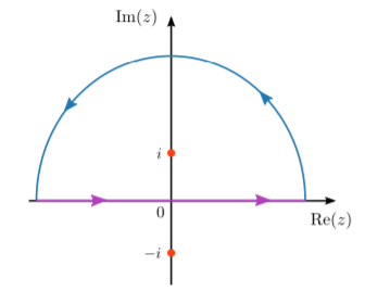
The resulting loop contour encloses the pole at \(z = +i\), so \[\oint \frac{dz}{z^2+1} = 2\pi i \; \mathrm{Res}\left[\frac{1}{z^2 + 1}\right]_{z = +i} = \pi.\] Note that the loop is counterclockwise, so we take the positive sign for the residue theorem. The loop integral can also be written as a sum of two integrals: \[\oint \frac{dz}{z^2 + 1} = \int_{-\infty}^\infty \frac{dx}{x^2 + 1} \;+\; \int_{\mathrm{arc}} \frac{dz}{z^2 + 1}.\] The first term is the integral we’re interested in. The second term, the contour integral along the arc, goes to zero. To see why, observe that along an arc of radius \(R\), the magnitude of the integrand goes as \(1/R^{2}\), while the \(dz\) gives another factor of \(R\) (see Section 9.1), so the overall integral goes as \(1/R\), which vanishes as \(R \rightarrow \infty\).
We thus obtain the result \[\int_{-\infty}^\infty \frac{dx}{x^2 + 1} = \pi.\] As an exercise, you can verify that closing the contour in the lower half-plane leads to exactly the same result.
Jordan’s lemma
Before proceeding to more complicated uses of contour integration, we must discuss an important result called Jordan’s lemma:
Theorem \(\PageIndex{1}\)
Let \[I = \int_C dz \; e^{iqz} \,g(z),\] where \(q\) is any positive real constant, and the contour \(C\) which is a semi-circular arc of radius \(R\) in the upper half-plane, centered at the origin. Then \[\text{If}\;\; \big|\,g(z)\,\big| < g_{\mathrm{max}} \;\;\;\text{for all}\;\;z \in C \;\;\;\Rightarrow \;\;\; I \rightarrow 0 \;\;\mathrm{as}\;\; g_{\mathrm{max}} \rightarrow 0.\]
In other words, if the factor of \(g(z)\) in the integrand does not blow up along the arc contour (i.e., its value is bounded), then in the limit where the bounding value goes to zero, the value of the entire integral vanishes.
Usually, the limiting case of interest is when the radius of the arc goes to infinity. Even if the integrand vanishes in that limit, it may not be obvious that the integral \(I\) vanishes, because the integration is taken along an arc of infinite length (so we have a \(0\times\infty\) sort of situation). Jordan’s lemma then proves useful, as it provides a set of criteria that can let us instantly conclude that \(I\) should vanish.
The proof for Jordan’s lemma is tedious, and we will not go into its details.
For integrands containing a prefactor of \(e^{-iqz}\) rather than \(e^{iqz}\) (again, where \(q \in \mathbb{R}^+\)), a different version of Jordan’s lemma holds, referring to a contour \(C'\) in the lower half-plane:
Theorem \(\PageIndex{2}\)
Let \[I = \int_C dz \; e^{-iqz} \,g(z),\] where \(q\) is any positive real constant, and the contour \(C\) which is a semi-circular arc of radius \(R\) in the lower half-plane, centered at the origin. Then \[\text{If}\;\; \big|\,g(z)\,\big| < g_{\mathrm{max}} \;\;\;\text{for all}\;\;z \in C \;\;\;\Rightarrow \;\;\; I \rightarrow 0 \;\;\mathrm{as}\;\; g_{\mathrm{max}} \rightarrow 0.\]
This is easily seen by doing the change of variable \(z \rightarrow -z\) on the original form of Jordan’s lemma.
As a convenient way to remember which variant of Jordan’s lemma to use, think about which end of imaginary axis causes the exponential factor to vanish: \[\begin{aligned} e^{iqz}\big|_{z = i\infty}\;\; = e^{-\infty} = 0\quad & \Rightarrow \;\; e^{iqz} \;\;\;\,\text{vanishes far above the origin}. \\ e^{-iqz}\big|_{z = -i\infty} = e^{-\infty} = 0\quad & \Rightarrow \;\; e^{-iqz} \;\;\textrm{vanishes far below the origin}.\end{aligned}\] Hence, for \(e^{iqz}\) (where \(q\) is any positive real number), the suppression occurs in the upper-half-plane. For \(e^{-iqz}\), the suppression occurs in the lower-half-plane.
A contour integral using Jordan’s lemma
Consider the integral \[I = \int_{-\infty}^\infty dx\; \frac{\cos(x)}{4x^2 + 1}.\] One possible approach is to break the cosine up into \((e^{ix} + e^{-ix})/2\), and do the contour integral on each piece separately. Another approach, which saves a bit of effort, is to write \[I = \mathrm{Re} \; \int_{-\infty}^\infty dx\; \frac{e^{ix}}{4x^2 + 1}.\] To do the integral, close the contour in the upper half-plane:

Then \[\oint dz \; \frac{e^{iz}}{4z^2 + 1} = \int_{-\infty}^\infty dx\; \frac{e^{ix}}{4x^2 + 1} + \int_{\mathrm{arc}} dz \; \frac{e^{iz}}{4z^2 + 1}.\] On the right-hand side, the first term is what we want. The second term is a counter-clockwise arc in the upper half-plane. According to Jordan’s lemma, this term goes to zero as the arc radius goes to infinity, since the rest of the integrand goes to zero for large \(|z|\): \[\left|\frac{1}{4z^2 + 1}\right| \sim \frac{1}{4|z|^2} \rightarrow 0 \quad \mathrm{as} \;|z| \rightarrow \infty.\] As for the loop contour, it can be evaluated using the residue theorem: \[\begin{align} \oint dz \; \frac{e^{iz}}{4z^2 + 1} &= \mathrm{Res}\left[\frac{e^{iz}}{4z^2 + 1}\right]_{\mathrm{enclosed}\;\mathrm{poles}}\\ &= 2\pi i \; \mathrm{Res}\left[\frac{1}{4}\, \frac{e^{iz}}{(z+i/2)(z-i/2)}\right]_{z = i/2} \\ &= 2\pi i \; \frac{e^{-1/2}}{4i}.\end{align}\] Hence, \[I = \mathrm{Re}\;\left[\frac{\pi}{2\sqrt{e}}\right]= \frac{\pi}{2\sqrt{e}}.\] In solving the integral this way, we must close the contour in the upper half-plane because our choice of complex integrand was bounded in the upper half-plane. Alternatively, we could have chosen to write \[I = \mathrm{Re} \; \int_{-\infty}^\infty dx\; \frac{e^{-ix}}{4x^2 + 1},\] i.e., with \(e^{-ix}\) rather than \(e^{ix}\) in the numerator. In that case, Jordan’s lemma tells us to close the contour in the lower half-plane. The arc in the lower half-plane vanishes, as before, while the loop contour is clockwise (contributing an extra minus sign) and encloses the lower pole: \[\begin{align} \oint dz \frac{e^{-iz}}{4z^2 + 1} &= -2\pi i \, \mathrm{Res}\left[ \frac{e^{-iz}}{4z^2 + 1} \right]_{z = -i/2} \\ &= - 2\pi i \frac{e^{-1/2}}{-4i} \\ &= \frac{\pi}{2\sqrt{e}}.\end{align}\] Taking the real part, we obtain the same result as before.
Principal value integrals
Sometimes, we come across integrals that have poles lying on the desired integration contour.
As an example, consider \[I = \int_{-\infty}^\infty dx\; \frac{\sin(x)}{x}.\] Because of the series expansion of the sine function, the integrand does not diverge at \(x = 0\), and the integral is in fact convergent. The integral can be solved without using complex numbers by using the arcane trick of differentiating under the integral sign (see Section 3.6). But it can also be solved straightforwardly via contour integration, with just a few extra steps.
We start by writing \[I = \mathrm{Im}(I'), \quad \mathrm{where}\;\;\; I' = \int_{-\infty}^\infty dx\; \frac{e^{ix}}{x}.\] We want to calculate \(I'\) with the help of contour integration. But there’s something strange about \(I'\): the complex integrand has a pole at \(z = 0\), right on the real line!
To handle this, we split \(I'\) into two integrals, one going over \(-\infty < x < -\epsilon\) (where \(\epsilon\) is some positive infinitesimal), and the other over \(\epsilon < x < \infty\): \[\begin{align} I' &= \lim_{\epsilon \rightarrow 0} \left[ \int_{-\infty}^{-\epsilon} dx\; \frac{e^{ix}}{x} + \int_{\epsilon}^\infty dx\; \frac{e^{ix}}{x}\right] \\ &\equiv \mathcal{P} \int_{-\infty}^\infty dx\; \frac{e^{ix}}{x}.\end{align}\] In the last line, the notation \(\mathcal{P}[\cdots]\) is short-hand for this procedure of “chopping away” an infinitesimal segment surrounding the pole. This is called taking the principal value of the integral.
Note
Even though this bears the same name as the “principal values” for multi-valued complex operations discussed in Chapter 8, there is no connection between the two concepts.
Now consider the loop contour shown in the figure below. The loop follows the principal-value contour along the real axis, skips over the pole at \(z = 0\) and arcs back along the upper half-plane. Since it encloses no poles, the loop integral vanishes by Cauchy’s integral theorem. However, the loop can also be decomposed into several sub-contours:
- \(\Gamma_1\), consisting of the segments along the real axis.
- \(\Gamma_2\), the large counter-clockwise semi-circular arc.
- \(\Gamma_3\), the infinitesimal clockwise semi-circular arc that skips around \(z = 0\).
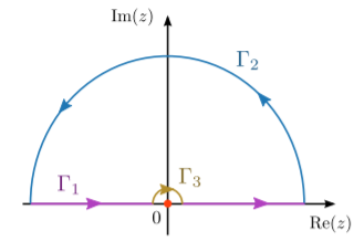
The integral over \(\Gamma_1\) is the principal-value integral we are interested in. The integral over \(\Gamma_2\) vanishes by Jordan’s lemma. The integral over \(\Gamma_3\) can be calculated by parameterization: \[\begin{align} \int_{\Gamma_3} \frac{e^{iz}}{z} &= \lim_{\epsilon \rightarrow 0} \int_{\pi}^{0} \frac{e^{i\epsilon \exp(i\theta)}}{\epsilon e^{i\theta}} \left(i\epsilon e^{i\theta}\right) d\theta \\ &= \lim_{\epsilon \rightarrow 0} i \int_{\pi}^0 d\theta \\ &= - i\pi.\end{align}\] Intutively, since encircling a pole anticlockwise gives a factor of \(2\pi i\) times the residue (which is 1 in this case), a clockwise semi-circle is associated with a factor of \(- i \pi\). Finally, putting everything together, \[\underbrace{\int_{\Gamma_1 + \Gamma_2 + \Gamma_3} f(z) dz}_{ =~0~(\text{Cauchy's integral theorem})} = \underbrace{\int_{\Gamma_1} f(z) dz}_{=~I'} + \underbrace{\int_{\Gamma_2} f(z) dz}_{=~0~(\text{Jordan's lemma})} + \underbrace{\int_{\Gamma_3} f(z) dz.}_{=~-i \pi}\] Hence, \[I = \mathrm{Im}(I') = \mathrm{Im}(i\pi) = \pi.\] This agrees with the result obtained by the method of differentiating under the integral sign from Section 3.6.
Alternatively, we could have chosen the loop contour so that it skips below the pole at \(z = 0\). In that case, the loop integral would be non-zero, and can be evaluated using the residue theorem. The final result is the same.