Transportation Problem | Set 2 (NorthWest Corner Method) - GeeksforGeeks

Transportation Problem | Set 2 (NorthWest Corner Method)

Last Updated : 09 Nov, 2023
Improve
Improve
Like Article
Like
Save
Share
Report

An introduction to Transportation problem has been discussed in the previous article, in this article, finding the initial basic feasible solution using the NorthWest Corner Cell Method will be discussed. 
 

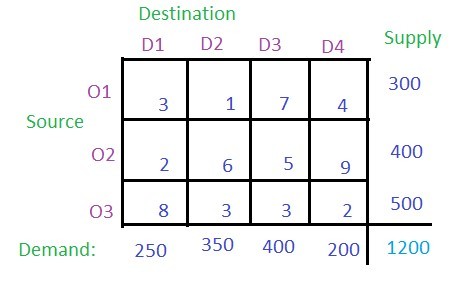
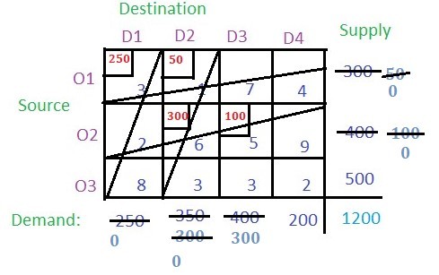
Explanation: Given three sources O1, O2 and O3 and four destinations D1, D2, D3 and D4. For the sources O1, O2 and O3, the supply is 300, 400 and 500 respectively. The destinations D1, D2, D3 and D4 have demands 250, 350, 400 and 200 respectively. 
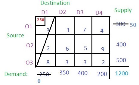
Solution: According to North West Corner method, (O1, D1) has to be the starting point i.e. the north-west corner of the table. Each and every value in the cell is considered as the cost per transportation. Compare the demand for column D1 and supply from the source O1 and allocate the minimum of two to the cell (O1, D1) as shown in the figure. 
The demand for Column D1 is completed so the entire column D1 will be canceled. The supply from the source O1 remains 300 – 250 = 50

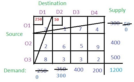
Now from the remaining table i.e. excluding column D1, check the north-west corner i.e. (O1, D2) and allocate the minimum among the supply for the respective column and the rows. The supply from O1 is 50 which is less than the demand for D2 (i.e. 350), so allocate 50 to the cell (O1, D2). Since the supply from row O1 is completed cancel the row O1. The demand for column D2 remain 350 – 50 = 300
 

From the remaining table the north-west corner cell is (O2, D2). The minimum among the supply from source O2 (i.e 400) and demand for column D2 (i.e 300) is 300, so allocate 300 to the cell (O2, D2). The demand for the column D2 is completed so cancel the column and the remaining supply from source O2 is 400 – 300 = 100
 

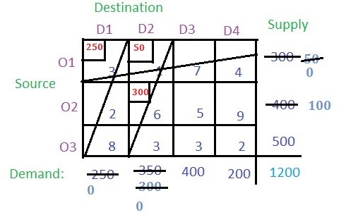
Now from remaining table find the north-west corner i.e. (O2, D3) and compare the O2 supply (i.e. 100) and the demand for D2 (i.e. 400) and allocate the smaller (i.e. 100) to the cell (O2, D2). The supply from O2 is completed so cancel the row O2. The remaining demand for column D3 remains 400 – 100 = 300
 

Proceeding in the same way, the final values of the cells will be: 
 

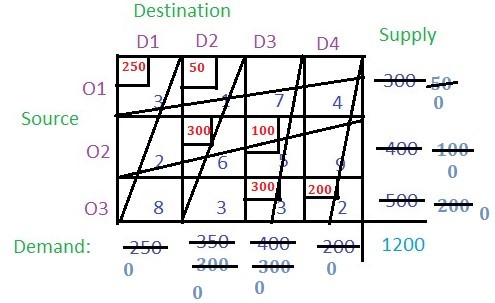
Note: In the last remaining cell the demand for the respective columns and rows are equal which was cell (O3, D4). In this case, the supply from O3 and the demand for D4 was 200 which was allocated to this cell. At last, nothing remained for any row or column. 
Now just multiply the allocated value with the respective cell value (i.e. the cost) and add all of them to get the basic solution i.e. (250 * 3) + (50 * 1) + (300 * 6) + (100 * 5) + (300 * 3) + (200 * 2) = 4400

Below is the implementation of the above approach

C++


#include <iostream>
#include <vector>
 
int main() {
    std::vector<std::vector<int>> grid = {{3, 1, 7, 4}, {2, 6, 5, 9}, {8, 3, 3, 2}}; // table
    std::vector<int> supply = {300, 400, 500}; // supply
    std::vector<int> demand = {250, 350, 400, 200}; // demand
 
    int startR = 0; // start row
    int startC = 0; // start col
    int ans = 0;
    // loop runs until it reaches the bottom right corner
    while (startR != grid.size() && startC != grid[0].size()) {
        // if demand is greater than supply
        if (supply[startR] <= demand[startC]) {
            ans += supply[startR] * grid[startR][startC];
            // subtract the value of supply from the demand
            demand[startC] -= supply[startR];
            startR += 1;
        }
        // if supply is greater than demand
        else {
            ans += demand[startC] * grid[startR][startC];
            // subtract the value of demand from the supply
            supply[startR] -= demand[startC];
            startC += 1;
        }
    }
 
    std::cout << "The initial feasible basic solution is " << ans << std::endl;
 
    return 0;
}


Java


public class GFG {
    public static void main(String[] args)
    {
        int[][] grid = new int[][] {
            { 3, 1, 7, 4 }, { 2, 6, 5, 9 }, { 8, 3, 3, 2 }
        }; // table
 
        int[] supply
            = new int[] { 300, 400, 500 }; // supply
        int[] demand
            = new int[] { 250, 350, 400, 200 }; // demand
 
        int startR = 0; // start row
        int startC = 0; // start col
        int ans = 0;
 
        // Loop runs until it reaches the bottom right
        // corner
        while (startR != grid.length
               && startC != grid[0].length) {
 
            // If demand is greater than supply
            if (supply[startR] <= demand[startC]) {
                ans += supply[startR]
                       * grid[startR][startC];
 
                // Subtract the value of supply from the
                // demand
                demand[startC] -= supply[startR];
                startR++;
            }
 
            // If supply is greater than demand
            else {
                ans += demand[startC]
                       * grid[startR][startC];
 
                // Subtract the value of demand from the
                // supply
                supply[startR] -= demand[startC];
                startC++;
            }
        }
 
        System.out.println(
            "The initial feasible basic solution is "
            + ans);
    }
}


Python3


grid = [[3, 1, 7, 4], [2, 6, 5, 9], [8, 3, 3, 2]]  # table
supply = [300, 400, 500# supply
demand = [250, 350, 400, 200# demand
 
startR = 0  # start row
startC = 0  # start col
ans = 0
# loop runs until it reaches the bottom right corner
while(startR != len(grid) and startC != len(grid[0])):
    # if demand is greater than supply
    if(supply[startR] <= demand[startC]):
        ans += supply[startR] * grid[startR][startC]
        # subtract the value of supply from the demand
        demand[startC] -= supply[startR]
        startR += 1
    # if supply is greater than demand
    else:
        ans += demand[startC] * grid[startR][startC]
        # subtract the value of demand from the supply
        supply[startR] -= demand[startC]
        startC += 1
 
print("The initial feasible basic solution is ", ans)


C#


using System;
 
class GFG {
  public static void Main(string[] args)
  {
 
    int[, ] grid = new int[3, 4] {
      { 3, 1, 7, 4 }, { 2, 6, 5, 9 }, { 8, 3, 3, 2 }
    }; // table
    int[] supply
      = new int[3] { 300, 400, 500 }; // supply
    int[] demand
      = new int[4] { 250, 350, 400, 200 }; // demand
 
    int startR = 0; // start row
    int startC = 0; // start col
    int ans = 0;
 
    // loop runs until it reaches the bottom right
    // corner
    while (startR != grid.GetLength(0)
           && startC != grid.GetLength(1))
    {
       
      // if demand is greater than supply
      if (supply[startR] <= demand[startC]) {
        ans += supply[startR]
          * grid[startR, startC];
 
        // subtract the value of supply from the
        // demand
        demand[startC] -= supply[startR];
        startR++;
      }
       
      // if supply is greater than demand
      else {
        ans += demand[startC]
          * grid[startR, startC];
 
        // subtract the value of demand from the
        // supply
        supply[startR] -= demand[startC];
        startC++;
      }
    }
 
    Console.WriteLine(
      "The initial feasible basic solution is "
      + ans);
  }
}


Javascript


let grid = [[3, 1, 7, 4], [2, 6, 5, 9], [8, 3, 3, 2]]; // table
let supply = [300, 400, 500]; // supply
let demand = [250, 350, 400, 200]; // demand
 
let startR = 0; // start row
let startC = 0; // start col
let ans = 0;
 
// loop runs until it reaches the bottom right corner
while (startR !== grid.length && startC !== grid[0].length)
{
 
  // if demand is greater than supply
  if (supply[startR] <= demand[startC])
  {
    ans += supply[startR] * grid[startR][startC];
     
    // subtract the value of supply from the demand
    demand[startC] -= supply[startR];
    startR += 1;
  }
   
  // if supply is greater than demand
  else
  {
    ans += demand[startC] * grid[startR][startC];
     
    // subtract the value of demand from the supply
    supply[startR] -= demand[startC];
    startC += 1;
  }
}
 
console.log("The initial feasible basic solution is " + ans);


Output

The initial feasible basic solution is  4400


Similar Reads

Transportation Problem | Set 7 ( Degeneracy in Transportation Problem )
Please go through this article first. This article will discuss degeneracy in transportation problem through an explained example. Solution: This problem is balanced transportation problem as total supply is equal to total demand. Initial basic feasible solution: Least Cost Cell Method will be used here to find the initial basic feasible solution.
3 min read
Transportation Problem | Set 6 (MODI Method - UV Method)
There are two phases to solve the transportation problem. In the first phase, the initial basic feasible solution has to be found and the second phase involves optimization of the initial basic feasible solution that was obtained in the first phase. There are three methods for finding an initial basic feasible solution, NorthWest Corner MethodLeast
7 min read
Transportation Problem | Set 3 (Least Cost Cell Method)
The North-West Corner method has been discussed in the previous article. In this article, the Least Cost Cell method will be discussed. Solution: According to the Least Cost Cell method, the least cost among all the cells in the table has to be found which is 1 (i.e. cell (O1, D2)). Now check the supply from the row O1 and demand for column D2 and
2 min read
Transportation Problem | Set 4 (Vogel's Approximation Method)
The North-West Corner method and the Least Cost Cell method has been discussed in the previous articles. In this article, the Vogel's Approximation method will be discussed. Solution: For each row find the least value and then the second least value and take the absolute difference of these two least values and write it in the corresponding row dif
14 min read
Transportation Problem Set 8 | Transshipment Model-1
Transshipment Model is a model which comes under the transportation problem. There are two types of transshipment problem: With sources and destination acting as transient (i.e. intermediary) nodesWith some transient nodes between sources and destination Look at the given transportation problem diagram. In a transportation problem, the shipment mov
3 min read
Transportation Problem | Set 5 ( Unbalanced )
An introduction to the transportation problem has been discussed in this article. In this article, the method to solve the unbalanced transportation problem will be discussed. Below transportation problem is an unbalanced transportation problem. The problem is unbalanced because the sum of all the supplies i.e. O1 , O2 , O3 and O4 is not equal to t
1 min read
Transportation Problem | Set 1 (Introduction)
Transportation problem is a special kind of Linear Programming Problem (LPP) in which goods are transported from a set of sources to a set of destinations subject to the supply and demand of the sources and destination respectively such that the total cost of transportation is minimized. It is also sometimes called as Hitchcock problem. Types of Tr
2 min read
Find the maximum cost path from the bottom-left corner to the top-right corner
Given a two dimensional grid, each cell of which contains integer cost which represents a cost to traverse through that cell. The task is to find the maximum cost path from the bottom-left corner to the top-right corner.Note: Use up and right moves only Examples: Input : mat[][] = {{20, -10, 0}, {1, 5, 10}, {1, 2, 3}} Output : 18 (2, 0) ==&gt; (2,
9 min read
Maximize sum of atmost K elements in array by taking only corner elements | Set 2
Given an array arr[] and an integer K, the task is to find and maximize the sum of at most K elements in the Array by taking only corner elements. A corner element is an element from the start of the array or from the end of the array. Examples: Input: N = 8, arr[] = {6, -1, 14, -15, 2, 1, 2, -5}, K = 4 Output: 19 Explanation: Here the optimal choi
12 min read
Secretary Problem (A Optimal Stopping Problem)
The Secretary Problem also known as marriage problem, the sultan's dowry problem, and the best choice problem is an example of Optimal Stopping Problem. This problem can be stated in the following form: Imagine an administrator who wants to hire the best secretary out of n rankable applicants for a position. The applicants are interviewed one by on
12 min read
Practice Tags :