Comment on “Theoretical examination of QED Hamiltonian in relativistic molecular orbital theory” [J. Chem. Phys. 159, 054105 (2023)]

Liu, Wenjian

doi:10.1063/5.0174011

In a recent paper (called Paper I hereafter),¹ Inoue and co-workers sifted in total nine quantum electrodynamics (QED) Hamiltonians resulting from combinations of three types of contractions of fermion operators [constantly null contraction (CNC),¹ charge-conjugated contraction (CCC),² and conventional contraction (cC); vide post] and three representations of the vacuum [free-particle orbitals (FPO), Furry orbitals (FO), and molecular orbitals (MO)], based on four criteria (orbital rotation invariance, charge conjugation invariance, time reversal invariance, and nonrelativistic limit). The term “nonrelativistic limit” (nrl) means here that, in the limit of the infinite speed of light, a correct QED Hamiltonian should agree with the nonrelativistic one for a system composed of both electrons and (real) positrons. Their conclusion was that only the MO-CNC variant $(H_{n}^{Q E D (M O - C N C)})$ of the nine QED Hamiltonians, along with the MOs that give a stationary point of total energy and a counter term that suppresses divergence, is free of internal inconsistence and is hence the recommended QED Hamiltonian. However, the $H_{n}^{Q E D (M O - C N C)}$ Hamiltonian [also called Fock-space (FS) Hamiltonian³] misses by construction the leading QED effect [vacuum polarization (VP) and electron self-energy (ESE)], at variance with the complete $H_{n}^{Q E D (M O - C C C)}$ Hamiltonian.² In addition, some of their manipulations are inconsistent and even incorrect such that their recommendation should be revised.

To expedite subsequent manipulations, the following conventions are to be adopted: (1) occupied and unoccupied positive-energy spinors (PES) are denoted by {i, j, …} and {a, b, …}, respectively; (2) occupied and general negative-energy spinors (NES) are denoted by ${\tilde{i}, \tilde{j}, \dots}$ and ${\tilde{p}, \tilde{q}, \tilde{r}, \tilde{s}}$ ⁠, respectively; (3) general spinors are denoted by {p, q, r, s, …}; (4) the Einstein summation convention over repeated indices is always employed.

The point of departure is the second-quantized relativistic Hamiltonian,

\begin{align} H & = \int {\hat{ϕ}}^{†} (r) D \hat{ϕ} (r) d r^{3} + \frac{1}{2} \iint {\hat{ϕ}}^{†} (r_{1}) {\hat{ϕ}}^{†} (r_{2}) \\ \times V (r_{12}) \hat{ϕ} (r_{2}) \hat{ϕ} (r_{1}) d r_{1}^{3} d r_{2}^{3} . \end{align}

(1)

To be in line with the filled Dirac picture, we write the Dirac matter field

\hat{ϕ} (r)

as^2,4

\hat{ϕ} (r) = a_{p} ψ_{p} (r) + a_{\tilde{p}} ψ_{\tilde{p}} (r), p \in P E S, \tilde{p} \in N E S,

(2)

along with the “vacuum”

| 0; \tilde{N} 〉 = Π_{\tilde{i} = 1}^{\tilde{N}} a^{\tilde{i}} | 0; \tilde{0} 〉, a_{p} | 0; \tilde{N} 〉 = a^{\tilde{p}} | 0; \tilde{N} 〉 = 0 .

(3)

Here, the spinors

{ψ_{p}}_{p = 1}^{2 \tilde{N}}

are eigenfunctions of the following mean-field Dirac equation (in atomic units):

f ψ_{p} = ϵ_{p} ψ_{p}, p \in P E S, N E S,

(4)

f = D + U, D = c α \cdot p + β c^{2} + V_{nuc} .

(5)

Plugging expression into Eq. leads to

H = D_{p}^{q} a_{q}^{p} + \frac{1}{2} g_{p r}^{q s} a_{q s}^{p r}, p, q, r, s \in PES, NES,

(6)

D_{p}^{q} = ⟨ ψ_{p} | D | ψ_{q} ⟩, g_{p r}^{q s} = (ψ_{p} ψ_{q} | V (r_{12}) | ψ_{r} ψ_{s}),

(7)

a_{q}^{p} = a^{p} a_{q}, a_{q s}^{p r} = a^{p} a^{r} a_{s} a_{q}, a^{p} = a_{p}^{†} .

(8)

Since the internal energy of the

\tilde{N}

occupied NES [cf. Eq. ] is not observable, we must normal order the Hamiltonian

H

with respect to the “vacuum”

| 0; \tilde{N} 〉

so as to obtain the physical Hamiltonian

H_{n}^{Q E D (M O)}

⁠,

H_{n}^{Q E D (M O)} = H - C_{n}

(9)

= H_{n}^{F S (M O)} + Q_{p}^{q} {a_{q}^{p}}_{n},

(10)

H_{n}^{F S (M O)} = D_{p}^{q} {a_{q}^{p}}_{n} + \frac{1}{2} g_{p q}^{r s} {a_{r s}^{p q}}_{n}, p, q, r, s \in PES, NES,

(11)

(12)

C_{n} = ⟨ 0; \tilde{N} | H | 0; \tilde{N} ⟩

(13)

(14)

through the following relations:

(15a)

(15b)

The crucial point here is how to define the contractions

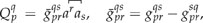
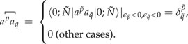
. Paper I compared the following three contraction schemes:

Constantly null contraction (CNC),¹
(16)
Charge-conjugated contraction (CCC),²
(17)
$\begin{align} = \frac{1}{2} ⟨ 0; \tilde{N} | a^{\tilde{p}} a_{\tilde{q}} | 0; \tilde{N} ⟩ |_{ϵ_{\tilde{p}} < 0, ϵ_{\tilde{q}} < 0} \\ - \frac{1}{2} ⟨ 0; \tilde{N} | a_{q} a^{p} | 0; \tilde{N} ⟩ |_{ϵ_{p} > 0, ϵ_{q} > 0} \end{align}$
(18)
$= - \frac{1}{2} δ_{q}^{p} sgn (ϵ_{q}), p, q \in PES, NES .$
(19)
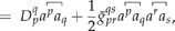
Conventional contraction (cC),
(20)
It is then clear that scheme (I) leads to
$H_{n}^{Q E D (M O - C N C)} = H_{n}^{F S (M O)},$
(21)
$Q_{p}^{q} = 0, C_{n} = 0,$
(22)
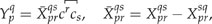
scheme (II) leads to
$H_{n}^{Q E D (M O - C C C)} = H_{n}^{F S (M O)} + Q_{p}^{q} {a_{q}^{p}}_{n},$
(23)
$Q_{p}^{q} = {\tilde{Q}}_{p}^{q} + {\bar{Q}}_{p}^{q} = - \frac{1}{2} {\bar{g}}_{p s}^{q s} sgn (ϵ_{s}),$
(24)
${\tilde{Q}}_{p}^{q} = - \frac{1}{2} g_{p s}^{q s} sgn (ϵ_{s}),$
(25)
${\bar{Q}}_{p}^{q} = \frac{1}{2} g_{p s}^{s q} sgn (ϵ_{s}),$
(26)
$\begin{align} C_{n} & = - \frac{1}{2} D_{p}^{p} sgn (ϵ_{p}) + \frac{1}{8} {\bar{g}}_{p q}^{p q} sgn (ϵ_{p}) sgn (ϵ_{q}) \\ = - \frac{1}{2} D_{p}^{p} sgn (ϵ_{p}) - \frac{1}{4} Q_{p}^{p} sgn (ϵ_{p}), \end{align}$
(27)
whereas scheme (III) gives rise to
$H_{n}^{Q E D (M O - c C)} = H_{n}^{F S (M O)} + Q_{p}^{q} {a_{q}^{p}}_{n},$
(28)
$Q_{p}^{q} = {\bar{g}}_{p \tilde{i}}^{q \tilde{i}},$
(29)
$C_{n} = D_{\tilde{i}}^{\tilde{i}} + \frac{1}{2} {\bar{g}}_{\tilde{i} \tilde{j}}^{\tilde{i} \tilde{j}} .$
(30)

The Q-potential in Eq. (29) is infinitely repulsive for positive-energy electrons $(\tilde{N} \to \infty)$ ⁠, meaning that no atom would be stable, just like the empty Dirac picture. As such, $H_{n}^{Q E D (M O - c C)}$ (28) should be rejected from the outset. In contrast, the Q-potential in Eq. (24) arising from scheme (II) is composed precisely of the VP in Eq. (25) and ESE in Eq. (26) (NB: the frequency-dependent transverse-photon interaction has to be included in ${\bar{Q}}_{p}^{q}$ to make the ESE complete⁵). Scheme (I) ignores such a genuine QED effect completely. Because of this, the so-called QED effect in Paper I refers actually to the correlation aspect of NES that was first surveyed in Ref. 4. As a matter of fact, $H_{n}^{Q E D (M O - C N C)}$ (21) is nothing but the Fock-space (FS) Hamiltonian $H_{n}^{F S (M O)}$ (11) advocated by Kutzelnigg,³ who missed simultaneous contractions between photon lines and between fermion lines when constructing $H_{n}^{F S (M O)}$ (11) in a diagrammatic derivation.⁶

Expression , along with the “vacuum” , is of course equivalent to the usual QED prescription of the Dirac matter field

\hat{ϕ} (r) = b_{p} ψ_{p} (r) + b^{\tilde{p}} ψ_{\tilde{p}} (r),

(31)

through the mapping

a_{p} \to b_{p}, a_{\tilde{p}} \to b^{\tilde{p}}, | 0; \tilde{N} 〉 \to | 0; \tilde{0} 〉 .

(32)

Operationally, expression (31) is merely a particle–hole reinterpretation of Eq. (2) [i.e., the creation of a hole of charge +1 via $a_{\tilde{p}} | 0; \tilde{N} 〉$ is equivalent to the creation of a positive-energy positron via $b^{\tilde{p}} | 0; \tilde{0} 〉$ ⁠, and both $a_{p} | 0; \tilde{N} 〉$ and $b_{p} | 0; \tilde{0} 〉$ annihilate a positive-energy electron] and is useful mainly in diagrammatic manipulations.⁶ In contrast, working with the a-operators is algebraically much simpler. Nevertheless, working with the b-operators will make the symmetric treatment of the electron and positron negative-energy seas by schemes (I) and (II) more transparent: the former neglects them completely, whereas the latter accounts for them properly (see Ref. 7 for a thorough analysis). That is, both $H_{n}^{Q E D (M O - C N C)}$ and $H_{n}^{Q E D (M O - C C C)}$ are charge conjugation invariants, as demonstrated in great detail in Paper I (see also the Appendix). In contrast, scheme (III) obviously violates charge conjugation symmetry. In the absence of external magnetic fields, both $H_{n}^{Q E D (M O - C N C)}$ and $H_{n}^{Q E D (M O - C C C)}$ commute with the time reversal operation. As such, they are also time reversal invariant as shown in Paper I.

The above normal-ordered Hamiltonians

H_{n}^{Q E D (M O - C N C)}

and

H_{n}^{Q E D (M O - C C C)}

were somehow rewritten in Paper I in unordered forms through relations . For instance, their Eq. reads in the present notation as

\begin{align} H_{n}^{Q E D (M O - C N C)} & = D_{p}^{q} a_{q}^{p} + \frac{1}{2} g_{p r}^{q s} a_{q s}^{p r} + Q_{p}^{q} a_{q}^{p} - C_{n}, \\ p, q, r, s \in PES, NES, \end{align}

(33)

Q_{p}^{q} = - {\bar{g}}_{p \tilde{i}}^{q \tilde{i}},

(34)

C_{n} = D_{\tilde{i}}^{\tilde{i}} - \frac{1}{2} {\bar{g}}_{\tilde{i} \tilde{j}}^{\tilde{i} \tilde{j}} .

(35)

Clearly, it is scheme (III), instead of the designated scheme (I), that was actually adopted in Paper I to obtain this expression. Such inconsistence dictates that their Eq. is not equivalent to their Eq. as they claimed. The latter (which is quoted from Refs. 7–11 and should have been written in normal-ordered form) is merely a rewriting of

H_{n}^{Q E D (M O - C N C)}

[actually

H_{n}^{F S (M O)}

] through mapping . Since the Q-potential in Eq. tends to be infinitely attractive for electrons, their expression [as well as Eqs. (33), (81), and (99) in Paper I] is not legitimate, just like Eq. . Moreover, their Eq. for

H_{n}^{Q E D (M O - C C C)}

also arises from the incorrect use of scheme (II). Specifically, according to the very definition of a normal-ordered Hamiltonian, their Eq. should have been written as

H_{n}^{Q E D (M O - C C C)} = H - C_{n}

⁠, with H and C_n defined in Eqs. and , respectively. These wrong expressions led them to conclude that neither

H_{n}^{Q E D (M O - C N C)}

/

H_{n}^{F S (M O)}

nor

H_{n}^{Q E D (M O - C C C)}

is orbital rotation invariant and that

H_{n}^{Q E D (M O - C C C)}

cannot reproduce the nonrelativistic Hamiltonian [Eq. (50) in Paper I] for both electrons and (real) positrons [cf. Eq. (59) in Paper I]. Since the (correct)

H_{n}^{Q E D (M O - C N C)}

/

H_{n}^{F S (M O)}

and

H_{n}^{Q E D (M O - C C C)}

are both in tensor form, they are certainly orbital rotation invariant according to tensor theory (see, e.g., Ref. 12). On the other hand, the nrl of

H_{n}^{Q E D (M O - C C C)}

[and

H_{n}^{F S (M O)}

] can readily be obtained as

\begin{align} H^{N R (M O - C C C))} & = h_{p q}^{(+)} {a_{q}^{p}}_{n} - h_{\tilde{p} \tilde{q}}^{(-)} {a_{\tilde{q}}^{\tilde{p}}}_{n} + \frac{1}{2} G_{p r}^{q s} {a_{q s}^{p r}}_{n} \\ + \frac{1}{2} G_{\tilde{p} \tilde{r}}^{\tilde{q} \tilde{s}} {a_{\tilde{q} \tilde{s}}^{\tilde{p} \tilde{r}}}_{n} + G_{p \tilde{r}}^{q \tilde{s}} {a_{q \tilde{s}}^{p \tilde{r}}}_{n}, \end{align}

(36)

by virtue of the following relations (see also Paper I):

ψ_{p} = (\begin{matrix} ψ_{p}^{L} \\ ψ_{p}^{S} \end{matrix}) \overset{c \to \infty}{\to} (\begin{matrix} ϕ_{p} \\ \frac{1}{2 c} σ \cdot p ϕ_{p} \end{matrix}),

(37)

ψ_{\tilde{p}} = (\begin{matrix} ψ_{\tilde{p}}^{L} \\ ψ_{\tilde{p}}^{S} \end{matrix}) \overset{c \to \infty}{\to} (\begin{matrix} - \frac{1}{2 c} σ \cdot p ϕ_{\tilde{p}} \\ ϕ_{\tilde{p}} \end{matrix}),

(38)

ψ_{p}^{†} (r) ψ_{\tilde{q}} (r) \overset{c \to \infty}{\to} 0, ψ_{\tilde{p}}^{†} (r) ψ_{q} (r) \overset{c \to \infty}{\to} 0,

(39)

〈 ψ_{p} | D - β c^{2} | ψ_{q} 〉 \overset{c \to \infty}{\to} h_{p q}^{(+)} = \frac{1}{2} 〈 ϕ_{p} | p^{2} | ϕ_{q} 〉 + 〈 ϕ_{p} | V_{nuc} | ϕ_{q} 〉,

(40)

〈 ψ_{\tilde{p}} | D + β c^{2} | ψ_{\tilde{q}} 〉 \overset{c \to \infty}{\to} - h_{\tilde{p} \tilde{q}}^{(-)}, h_{\tilde{p} \tilde{q}}^{(-)} = \frac{1}{2} 〈 ϕ_{\tilde{p}} | p^{2} | ϕ_{\tilde{q}} 〉 - 〈 ϕ_{\tilde{p}} | V_{nuc} | ϕ_{\tilde{q}} 〉,

(41)

g_{p r}^{q s} \overset{c \to \infty}{\to} G_{p r}^{q s} = (ϕ_{p} ϕ_{q} | ϕ_{r} ϕ_{s}),

(42)

g_{\tilde{p} \tilde{r}}^{\tilde{q} \tilde{s}} \overset{c \to \infty}{\to} G_{\tilde{p} \tilde{r}}^{\tilde{q} \tilde{s}} = (ϕ_{\tilde{p}} ϕ_{\tilde{q}} | ϕ_{\tilde{r}} ϕ_{\tilde{s}}),

(43)

g_{p \tilde{r}}^{q \tilde{s}} \overset{c \to \infty}{\to} G_{p \tilde{r}}^{q \tilde{s}} = (ϕ_{p} ϕ_{q} | ϕ_{\tilde{r}} ϕ_{\tilde{s}}),

(44)

Q_{p}^{q} \overset{c \to \infty}{\to} 0, p, q \in P E S, N E S .

(45)

Here, {ϕ_p} and

{ϕ_{\tilde{p}}}

represent real-valued, nonrelativistic electronic and positronic states, respectively. Since the (full and renormalized) Q term represents the lowest-order QED effect [of order (Zα)³], it does not exist in the nrl, as implied by Eq. . Furthermore, using the following mapping [cf. Eq. ]:

{a_{\tilde{q}}^{\tilde{p}}}_{n} = - a_{\tilde{q}} a^{\tilde{p}} \to - b^{\tilde{q}} b_{\tilde{p}},

(46)

as well as permutation symmetries of the integrals (e.g.,

h_{\tilde{p} \tilde{q}}^{(-)} = h_{\tilde{q} \tilde{p}}^{(-)}

⁠), Eq. can be rewritten as

\begin{align} H^{N R (M O - C C C))} & = h_{p q}^{(+)} a^{p} a_{q} + h_{\tilde{p} \tilde{q}}^{(-)} b^{\tilde{p}} b_{\tilde{q}} + \frac{1}{2} G_{p r}^{q s} a^{p} a^{r} a_{s} a_{q} \\ + \frac{1}{2} G_{\tilde{p} \tilde{r}}^{\tilde{q} \tilde{s}} b^{\tilde{p}} b^{\tilde{r}} b_{\tilde{s}} b_{\tilde{q}} - G_{p \tilde{r}}^{q \tilde{s}} a^{p} a_{q} b^{\tilde{r}} b_{\tilde{s}}, \end{align}

(47)

which is obviously identical to Eq. of Paper I, at variance with their Eq. (59), that originates from the incorrect Eq. . As a matter of fact, the correct nrl of

H_{n}^{Q E D (M O - C C C)}

[and

H_{n}^{F S (M O)}

] should have been anticipated from the outset, for it treats electrons and positrons on an equal footing (see Sec. IV B of Ref. 7). Different from this, the nonrelativistic Hamiltonian H^NR(MO−CCC) describes electrons and positrons differently (the first and third terms vs the second and fourth terms) and couples them only by their charge attraction (the fifth term).

Given the QED Hamiltonian

H_{n}^{Q E D (M O - C C C)}

, the physical energy E of an N-electron system can be calculated as⁵

E = ⟨ Ψ (N; \tilde{N}) | H_{n}^{Q E D (M O - C C C)} | Ψ (N; \tilde{N}) ⟩

(48)

= ⟨ Ψ (N; \tilde{N}) | H | Ψ (N; \tilde{N}) ⟩ - ⟨ 0; \tilde{N} | H | 0; \tilde{N} ⟩ .

(49)

Equation [or Eq. (27) in Ref. 5] was criticized by Paper I, by saying that the second term [defined in Eq. ] cannot remove the divergence of the first term due to no correlation in the former. However, this is a complete misunderstanding. The second term of Eq. arises naturally from the definition of a normal-ordered Hamiltonian [see Eqs. and ]. Literally, its role is merely to remove the unobservable ingredient (internal energy of the negative-energy electrons) of

H

in the filled Dirac picture. Note, in particular, that the occupied PES are treated here as particles, just like the unoccupied PES. It becomes more transparent when going to a diagrammatic representation (see Fig. 4 in Ref. 2). It is lengthy but straightforward to evaluate the right-hand side of Eq. without referring explicitly to the reference

| 0; \tilde{N} 〉

(cf. the linked theorem of many-body theory¹³), just like the S-matrix formulation of QED [see Sec. II B 2 in Ref. 2). Of course, it is operationally much simpler to treat the occupied PES also as holes along with the occupied NES so as to calculate the energy as^2,4,5

E = 〈 Ψ (N; \tilde{N}) | H | Ψ (N; \tilde{N}) 〉 - 〈 Ψ (0; \tilde{N}) | H | Ψ (0; \tilde{N}) 〉 .

(50)

Pictorially, being in the same space, the occupied PES and NES can polarize each other so as to create responses of $Ψ (0; \tilde{N})$ ⁠, i.e., $Ψ (0; \tilde{N}) = Ψ^{(0)} (0; \tilde{N}) + Ψ^{(1)} (0; \tilde{N}) + \dots$ ⁠. More specifically, the first term of Eq. (50) contains the usual $a_{m}^{a}$ and $a_{m n}^{a b}$ $(m, n = i, j, \tilde{i}, \tilde{j})$ excitations but no $a_{\tilde{i}}^{i}$ or $a_{\tilde{i} \tilde{j}}^{i p}$ (p = j, a) type of excitations. The latter do appear in the first term of Eqs. (48)/(49) and must, hence, be accounted for by the second term of (50). The agreement between Eqs. (49) and (50) is ensured by the common zeroth-order setting, i.e., $| 0; \tilde{N} 〉 = Ψ^{(0)} (0; \tilde{N})$ ⁠. Since the second term of Eq. (50) appears naturally as a replacement of that of Eq. (49) (due to the change of the particle-to-hole character of the occupied PES), it need not be introduced in an a posteriori manner as performed in Paper I. Anyhow, it has long been known¹⁴ that the individual terms of Eq. (49)/(50) are divergent, but their difference is finite, such that the divergence problem (on the correlation contribution of NES) should not have been presented in Paper I as something new.

Equations / and give rise to the same second-order energy E⁽²⁾ for a system of N electrons as the S-matrix formulation of QED.² For comparison, we quote the special case of the general expression^2,5 for E⁽²⁾, with the effective potential U in Eq. set to the Hartree–Fock (HF) potential V_HF

(= {\bar{g}}_{\cdot j}^{\cdot j})

and the QED potential Q set to zero,

E^{(2)} = E_{1}^{(2)} + E_{2}^{(2)},

(51)

E_{1}^{(2)} = 0 - [\frac{{\bar{g}}_{\tilde{i} j}^{a j} {\bar{g}}_{a j}^{\tilde{i} j}}{ϵ_{\tilde{i}} - ϵ_{a}} + \frac{{\bar{g}}_{\tilde{i} j}^{i j} {\bar{g}}_{i j}^{\tilde{i} j}}{ϵ_{\tilde{i}} - ϵ_{i}}],

(52)

E_{2}^{(2)} = \frac{1}{4} \frac{{\bar{g}}_{m n}^{a b} {\bar{g}}_{a b}^{m n}}{ϵ_{m} + ϵ_{n} - ϵ_{a} - ϵ_{b}} |_{m, n = i, j, \tilde{i}, \tilde{j}} - \frac{1}{4} \frac{{\bar{g}}_{\tilde{i} \tilde{j}}^{p q} {\bar{g}}_{p q}^{\tilde{i} \tilde{j}}}{ϵ_{\tilde{i}} + ϵ_{\tilde{j}} - ϵ_{p} - ϵ_{q}} |_{p, q = i, j, a, b}

(53)

\begin{align} = [\frac{1}{4} \frac{{\bar{g}}_{i j}^{a b} {\bar{g}}_{a b}^{i j}}{ϵ_{i} + ϵ_{j} - ϵ_{a} - ϵ_{b}} + \frac{1}{2} \frac{{\bar{g}}_{i \tilde{j}}^{a b} {\bar{g}}_{a b}^{i \tilde{j}}}{ϵ_{i} + ϵ_{\tilde{j}} - ϵ_{a} - ϵ_{b}}] \\ - [\frac{1}{4} \frac{{\bar{g}}_{\tilde{i} \tilde{j}}^{i j} {\bar{g}}_{i j}^{\tilde{i} \tilde{j}}}{ϵ_{\tilde{i}} + ϵ_{\tilde{j}} - ϵ_{i} - ϵ_{j}} + \frac{1}{2} \frac{{\bar{g}}_{\tilde{i} \tilde{j}}^{i a} {\bar{g}}_{i a}^{\tilde{i} \tilde{j}}}{ϵ_{\tilde{i}} + ϵ_{\tilde{j}} - ϵ_{i} - ϵ_{a}}] . \end{align}

(54)

The first and second terms of Eqs. (52)/(53) correspond to the first and second terms of Eq. (50), respectively. While the two-body term $E_{2}^{(2)}$ (54) is identical to that in Eq. (95) of Paper I, the one-body term $E_{1}^{(2)}$ (52) is not present in the latter, where it was naively assumed that only double excitations contribute to E⁽²⁾. This is only true for the first term but not for the second term of Eq. (50). Since the HF potential V_HF arises only for systems of more than one positive-energy electron, it does not enter the second term of Eq. (50). As a result, the one-body perturbation $- {\bar{g}}_{p i}^{q i} {a_{q}^{p}}_{n}$ is not canceled out in the second term, unlike in the first term of Eq. (50) (see Ref. 7 for a detailed derivation).

So far, only the MO representation of the “vacuum” $| 0; \tilde{N} 〉$ has been considered. Other representations (e.g., FPO and FO⁵) are, of course, possible. However, different representations of the “vacuum” $| 0; \tilde{N} 〉$ amount just to setting the total energy to different zero points and hence do not introduce any new physics. Nevertheless, one should be aware that the known regularization/renormalization schemes in QED were designed only for local potentials [U in Eq. (5)]. Notwithstanding this, once the Q-potential (24) (along with the transverse-photon part of the ESE⁵) is fitted into a model operator,^15–17 the MO representation can safely be employed, which is much simpler [due to the cancellation of common terms between the first and second terms of Eq. (50)] and obviously more appropriate than other representations for molecular systems.

In summary, the $H_{n}^{Q E D (M O - C C C)}$ Hamiltonian (23) has passed trivially the test of all criteria raised in Paper I. In addition, it is more complete than $H_{n}^{Q E D (M O - C N C)}$ / $H_{n}^{F S (M O)}$ (11) (which is only part of the former). Since a bare (versus dressed) many-electron Hamiltonian is necessarily linear in the electron–electron interaction V(r₁₂), $H_{n}^{Q E D (M O - C C C)}$ is undoubtedly the most accurate relativistic Hamiltonian. As such, it is $H_{n}^{Q E D (M O - C C C)}$ instead of $H_{n}^{Q E D (M O - C N C)}$ / $H_{n}^{F S (M O)}$ that should be recommended. The following are some final remarks that are still pertinent to Paper I:

The same (multi-configurational) Dirack–Harfree–Fock equation can be derived from either the empty or filled Dirac picture, but only so when the Q-potential (24) is neglected [cf.Eq. (54) and subsequent discussions in Ref. 5].
Neglecting the leading (first-order) QED effect (VP-ESE) but accounting for the (at least second-order) contribution of NES to correlation is hardly meaningful.
The frequency-dependent Breit interaction has to be taken into account when evaluating the contribution of NES to correlation. Otherwise, it will be severely overestimated.¹⁸
Given the huge gap between the NES and PES, going beyond a second-order treatment of the NES is hardly necessary. Rather, the correlation within the manifold of PES is much harder (see Ref. 19 for effective means for simultaneous treatments of relativity, correlation, and QED).
Although the (full) Q-potential (24) can be fitted into a model operator,^15–17 it is still of great interest to test its convergence with respect to the size of Gaussian basis sets, a point that has not yet been surveyed before. The authors of Paper I are strongly encouraged to try this with their advanced coding.

This work was supported by the National Natural Science Foundation of China (Grant Nos. 22373057 and 21833001) and the Mount Tai Scholar Climbing Project of Shandong Province.

AUTHOR DECLARATIONS

Conflict of Interest

The author has no conflicts to disclose.

DATA AVAILABILITY

The data that support the findings of this study are available within the article.

APPENDIX: CHARGE CONJUGATION AND TIME REVERSAL (CT) TRANSFORMATIONS

The CT transformation of the QED Hamiltonians was demonstrated in great detail in Paper I. Here, we provide a more transparent manipulation. First of all, it can readily be shown that the charge conjugation transformation,

\hat{C} = C_{0} {\hat{K}}_{0}, {\hat{C}}^{†} = {\hat{C}}^{- 1} = \hat{C}, C_{0} = (\begin{matrix} 0_{2} & i σ_{y} \\ - i σ_{y} & 0_{2} \end{matrix}) = C_{0}^{†} = C_{0}^{- 1},

(A1)

of the mean-field Dirac Eq. leads to

f^{C} ψ_{p}^{C} = ϵ_{p}^{C} ψ_{p}^{C},

(A2)

f^{C} = - \hat{C} f {\hat{C}}^{- 1} = D^{C} - U, D^{C} = c α \cdot p + β m c^{2} - V_{nuc} = D^{C †},

(A3)

ψ_{p}^{C} = \hat{C} ψ_{p} = C_{0} ψ_{p}^{*}, ϵ_{p}^{C} = - ϵ_{p} .

(A4)

The

{\hat{K}}_{0}

operator in Eq. represents complex conjugation. The corresponding unitary transformation (denoted as

C

⁠) of the field operator

\hat{ϕ} (r)

gives²⁰

C \hat{ϕ} (r) C^{- 1} = {\hat{ϕ}}^{C} (r) = \hat{C} \hat{ϕ} (r) = b^{p} ψ_{p}^{C} (r) + b_{\tilde{p}} ψ_{\tilde{p}}^{C} (r),

(A5)

where the first term creates a positive-energy electron with probability

| ψ_{p}^{C} |^{2} = | ψ_{p} |^{2}

⁠, whereas the second term annihilates a positive-energy positron with probability

| ψ_{\tilde{p}}^{C} |^{2} = | ψ_{\tilde{p}} |^{2}

⁠, just opposite to the first and second terms of Eq. in terms of annihilations and creations [NB:

ϵ_{\tilde{p}}^{C} = - ϵ_{\tilde{p}} > 0

]. Put another way,

{\hat{ϕ}}^{C} (r)

is just the field operator for a world where positrons are regarded as particles and electrons are regarded as anti-particles, governed by the Hamiltonian f^C . It can also be rewritten as

{\hat{ϕ}}^{C} (r) = c^{p} ψ_{p}^{C} (r) + c^{\tilde{p}} ψ_{\tilde{p}}^{C} (r),

(A6)

provided that the vacuum

| 0; \tilde{0} 〉

underlying the form is replaced with

| 0; \tilde{N} 〉

⁠, for the actions of b^p and

b_{\tilde{p}}

on

| 0; \tilde{0} 〉

are the same as those of c^p and

c^{\tilde{p}}

on

| 0; \tilde{N} 〉

⁠.

Since the time reversal operator

\hat{T} = T_{0} {\hat{K}}_{0}, {\hat{T}}^{†} = \hat{T} = - {\hat{T}}^{- 1}, T_{0} = (\begin{matrix} - i σ_{y} & 0_{2} \\ 0_{2} & - i σ_{y} \end{matrix}) = T_{0}^{†} = - T_{0}^{- 1}

(A7)

commutes with both f and f^C , both the electronic

{ψ_{r}}_{r = 1}^{2 \tilde{N}}

and positronic eigen-spinors

{ψ_{p}^{C}}_{p = 1}^{2 \tilde{N}}

can be classified into Kramers pairs, i.e.,

{ψ_{k}, ψ_{\bar{k}} = T_{0} ψ_{k}^{*}}_{k = 1}^{\tilde{N}}

and

{ψ_{k}^{C}, ψ_{\bar{k}}^{C} = T_{0} ψ_{k}^{C *}}_{k = 1}^{\tilde{N}}

⁠, respectively. In particular,

ψ_{\bar{k}}^{C}

is related to ψ_k in a very simple way,

ψ_{\bar{k}}^{C} = \hat{T} \hat{C} ψ_{k} = T_{0} C_{0} ψ_{k} = {[T_{0} ψ_{k}^{C}]}^{*} = (\begin{matrix} ψ_{k}^{S} \\ - ψ_{k}^{L} \end{matrix}), k \in PES, NES .

(A8)

The antiunitary time reversal transformation (denoted as

T

⁠) of

{\hat{ϕ}}^{C} (r)

is defined as²⁰

T {\hat{ϕ}}^{C} (r, t) T^{- 1} = T_{0} {\hat{ϕ}}^{C} (r, - t) .

(A9)

Since we are only concerned with time-independent situations (stationary states), the time t in Eq. can simply be set to zero. We then have

\begin{align} {\hat{ϕ}}^{C T} (r) & = T_{0} {\hat{ϕ}}^{C} (r) \\ = b^{k} T_{0} ψ_{k}^{C} (r) + b^{\bar{k}} T_{0} ψ_{\bar{k}}^{C} (r) + b_{\tilde{k}} T_{0} ψ_{\tilde{k}}^{C} (r) + b_{\bar{\tilde{k}}} T_{0} ψ_{\bar{\tilde{k}}}^{C} (r) \end{align}

(A10)

= b^{k} ψ_{\bar{k}}^{C *} (r) - b^{\bar{k}} ψ_{k}^{C *} (r) + b_{\tilde{k}} ψ_{\bar{\tilde{k}}}^{C *} (r) - b_{\bar{\tilde{k}}} ψ_{\tilde{k}}^{C *} (r),

(A11)

where the use of relation has been made when going from Eq. to Eq. . The mismatch between the indices of the b-operators and their coefficients in Eq. can be resolved by the replacements (NB: a negative sign for two bars],

b^{k} \to d^{\bar{k}}, b^{\bar{k}} \to - d^{k}, b_{\tilde{k}} \to d_{\bar{\tilde{k}}}, b_{\bar{\tilde{k}}} \to - d_{\tilde{k}} .

(A12)

That is, Eq. should be rewritten as

{\hat{ϕ}}^{C T} (r) = d^{\bar{k}} ψ_{\bar{k}}^{C *} (r) + d^{k} ψ_{k}^{C *} (r) + d_{\bar{\tilde{k}}} ψ_{\bar{\tilde{k}}}^{C *} (r) + d_{\tilde{k}} ψ_{\tilde{k}}^{C *} (r)

(A13)

= d^{p} ψ_{p}^{C *} + d_{\tilde{p}} ψ_{\tilde{p}}^{C *}, p \in Kramers pairs

(A14)

for internal consistence. The legitimacy of transformation is very simple: Each term of Eq. is just an inner product between the row vector of basis operators and the column vector of expansion coefficients such that the indices for their elements must be aligned; a phase can be introduced to the element of a basis at will, for its coefficient will change accordingly. It follows that the following mapping:

b_{k} \to d^{\bar{k}}, ψ_{k} \to ψ_{\bar{k}}^{C *}, k \in P E S, N E S,

(A15a)

b_{\bar{k}} \to - d^{k}, ψ_{\bar{k}} \to ψ_{k}^{C *}, k \in P E S, N E S,

(A15b)

can be taken when going directly from field to the CT-transformed field . To expedite algebraic manipulations,

{\hat{ϕ}}^{C T} (r)

can further be rewritten as

{\hat{ϕ}}^{C T} (r) = c^{p} ψ_{p}^{C *} + c^{\tilde{p}} ψ_{\tilde{p}}^{C *}, p \in Kramers pairs,

(A16)

provided that the vacuum

| 0; \tilde{0} 〉

associated with

{\hat{ϕ}}^{C T} (r)

is replaced with

| 0; \tilde{N} 〉

⁠. The first of Eq. creates an electron via

c^{p} | 0; \tilde{N} 〉

(= d^{p} | 0; \tilde{0} 〉)

⁠, whereas the second term annihilates a positron via

c^{\tilde{p}} | 0; \tilde{N} 〉 = 0

(= d_{\tilde{p}} | 0; \tilde{0} 〉)

⁠, in line with those of Eq. .

Another point that should be noted is that both

C

and

T

act on state vectors (i.e., creation and annihilation operators). For instance, we have

C [A (r) \hat{ϕ} (r)] C^{- 1} = A^{C} (r) {\hat{ϕ}}^{C} (r), A^{C} (r) = \hat{C} A (r) {\hat{C}}^{- 1},

(A17)

T [A (r) \hat{ϕ} (r)] T^{- 1} = A^{*} (r) T_{0} \hat{ϕ} (r) .

(A18)

The complex conjugation of function A(r) in Eq. stems from the antilinearity of

T

⁠. Moreover, the following relations can readily be verified:

\hat{C} α {\hat{C}}^{- 1} = C_{0} α^{*} C_{0}^{- 1} = α, \hat{T} α {\hat{T}}^{- 1} = T_{0} α^{*} T_{0}^{- 1} = - α,

(A19)

ψ_{p}^{C †} ψ_{q}^{C} = ψ_{q}^{†} ψ_{p}, ψ_{\bar{p}}^{C †} ψ_{\bar{q}}^{C} = ψ_{p}^{†} ψ_{q},

(A20)

ψ_{p}^{C †} α ψ_{q}^{C} = ψ_{q}^{†} α ψ_{p}, ψ_{\bar{p}}^{C †} α ψ_{\bar{q}}^{C} = - ψ_{p}^{†} α ψ_{q} .

(A21)

In terms of the above entities, the CT transformation of the Hamiltonian

H

can readily found to be

H^{C T} = T C H C^{- 1} T^{- 1}

(A22)

\begin{align} = - \int {\hat{ϕ}}^{C T †} (r) D^{C *} {\hat{ϕ}}^{C T} (r) d r^{3} + \frac{1}{2} \iint {\hat{ϕ}}^{C T †} \\ \times (r_{1}) {\hat{ϕ}}^{C T †} (r_{2}) V^{*} (r_{12}) {\hat{ϕ}}^{C T} (r_{2}) {\hat{ϕ}}^{C T} (r_{1}) d r_{1}^{3} d r_{2}^{3} \end{align}

(A23)

= - c_{q} c^{p} x_{p}^{q} + \frac{1}{2} c_{q} c_{s} c^{r} c^{p} X_{p r}^{q s},

(A24)

x_{p}^{q} = ⟨ ψ_{p}^{C} | D^{C} | ψ_{q}^{C} ⟩ = - D_{q}^{p},

(A25)

X_{p r}^{q s} = (ψ_{p}^{C} ψ_{q}^{C} | V (r_{12}) | ψ_{r}^{C} ψ_{s}^{C}) = g_{q s}^{p r},

(A26)

where the summations run over all Kramers-paired PES and NES and the particle–particle interaction V(r₁₂) is assumed to commute with

\hat{C}

[which is true even in the presence of the Gaunt/Breit interaction; cf. the first equation in Eq. ]. The products of fermion operators in Eq. can be normal-ordered with respect to

| 0; \tilde{N} 〉

according to relations [e.g.,

so as to convert

H^{C T}

to

H^{C T} = H_{n}^{C T} + C_{n}^{C T},

(A27)

H_{n}^{C T} = x_{p}^{q} {c_{q}^{p}}_{n} + \frac{1}{2} X_{p r}^{q s} {c_{q s}^{p r}}_{n} + Y_{p}^{q} {c_{q}^{p}}_{n},

(A28)

(A29)

C_{n}^{C T} = ⟨ 0; \tilde{N} | H^{C T} | 0; \tilde{N} ⟩

(A30)

(A31)

It is clear that $H_{n}^{C T}$ (A28) and $H_{n}^{Q E D (M O)}$ (10) have the same functional form. That is, both $H_{n}^{Q E D (M O - C N C)}$ (21) [or rather $H_{n}^{F S (M O)}$ (11)] and $H_{n}^{Q E D (M O - C C C)}$ (23) are CT invariant.