Autoencoders in Practice: Dimensionality Reduction and Image Denoising
How to use autoencoders to reduce image dimension and the noise in an image with Python and TensorFlow

Autoencoder in a Nutshell
Let’s imagine ourselves creating a neural network based machine learning model. When we do so, most of the time we’re going to use it to do a classification task. This means that we train our neural network to predict the target y given the input features x.
However, the ability of a neural network to create a lower-dimensional representation of our data in a non-linear fashion opens up a lot of possibilities. Now we can train our neural network to compress our data and then decompress them back to their original dimension. This is the basic concept of an autoencoder.
In a nutshell, an autoencoder is a neural network based model to compress the data. Therefore, it has the ability to learn the compressed representation of our input data.
In the early development of Deep Learning, autoencoder has been viewed as a solution to solve the problem of unsupervised learning. This is because an autoencoder doesn’t really need a labeled ground-truth for it to learn the data.
However, it is important to note that an autoencoder itself is not a pure unsupervised learning technique. Autoencoder is a self-supervised learning technique, where the target that it needs to learn is generated from our input data. Let’s take a look at the code snippet below:
model.fit(x=x, y=x)Instead of using the model to predict the ground-truth label, as we usually do with supervised models, we use an autoencoder model to reconstruct our original input data to be as similar as possible. Because of that, the point of training an autoencoder is to minimize the so-called reconstruction loss. The lower the reconstruction loss, the more similar the reconstruction of the input data can be generated by the model.
In practice, you need two different functions to create an autoencoder model: an encoder and a decoder. These two functions are normally implemented with neural networks. It can be LSTM if you’re working on NLP use case, or Convolutional Neural Networks (CNN), if you’re working on Computer Vision use case.

As you can see above, there are three components of an autoencoder:
- Encoder — The function to compress the data to their lower-dimensional representation.
- Bottleneck — This is also called a latent space, where our initial data are now represented in a lower dimension.
- Decoder — The function to decompress or reconstruct our low dimension data back to their initial dimension.
Due to its encoder-decoder architecture, nowadays an autoencoder is mostly used in two of these domains: image denoising and dimensionality reduction for data visualization. In this article, let’s build an autoencoder to tackle these things.
Loading the Data
Before we start building an autoencoder, we need to load the data first. The data that we’re going to use is the Medical MNIST dataset. If you want to follow along, you can download the dataset here.

There are 58954 medical images belonging to 6 classes: AbdomenCT, BreastMRI, CXR, ChestCT, Hand, HeadCT. After downloading the data, unzip the file and place it in the directory of your choice. You should then have a folder with the following structure:
MedicalMNIST/    AbdomenCT/
    BreastMRI/
    CXR/
    ChestCT/
    Hand/
    HeadCT/
The next thing that we should do is to split the file into training and test folder. To do this, we can use a library called split-folders. You can install it by typing the following command:
pip install split-foldersWith this library, we can split our MedicalMNIST folder into training and test folder. We will allocate 80% of the data for training data and 20% for test data.
If you run the code above, now you get a new folder called ‘ MedicalMNIST_splitted‘. Inside this folder, you’ll see two folders: ‘training’ folder and ‘val’ folder. Your folder now should have the following structure.
MedicalMNIST_splitted/   train/
     AbdomenCT/
     BreastMRI/
     CXR/
     ChestCT/
     Hand/
     HeadCT/   val/
     AbdomenCT/
     BreastMRI/
     CXR/
     ChestCT/
     Hand/
     HeadCT/
Finally, we can generate our training and test data from these folders with image generator from TensorFlow.
If you run the code above, you’ll get your training and test data together with their ground-truth labels.
Now we are ready to build our autoencoder for dimensionality reduction and image denoising.
Autoencoder for Dimensionality Reduction
When we’re working on our machine learning projects, we commonly run into a problem where we have a lot of input variables. This means two things: first, your machine learning model will be likely to suffer from overfitting problem and second, you need to allocate a whole lot amount of time to train the model.
Dimensionality reduction is the technique that’ll save you from all of those problems. When dealing with a lot of input variables, it is often necessary to reduce the dimension of the data to capture the most valuable inputs among all of those input variables. Also, you can visualize your data and see how they occupy the latent space by lowering its dimension to two or three dimensions.
There are two techniques that are commonly used to reduce the dimension of your data: PCA and t-SNE. However, autoencoders can be used as well for dimensionality reduction.
In some cases, autoencoders perform even better than PCA because PCA can only learn linear transformation of the features. However, since autoencoders are built based on neural networks, they have the ability to learn the non-linear transformation of the features. This turns into a better reconstruction ability.
Let’s say we have two features, x1 and x2. In the first row, they have a linear relationship and in the second row, they have a non-linear relationship.

In the first row, since the two features have a linear relationship, then both PCA and autoencoders can accurately reconstruct the relationship between features in the latent space.
Meanwhile, if the two features have a non-linear relationship, as shown in the second row, then autoencoders would be more suited to use since they have the ability to learn non-linear relationship between features.
Building the Autoencoder Model
Now it’s time for us to build an autoencoder to reduce the dimension of our Medical MNIST images into two dimensions. After we reduce the dimension, we can visualize how our images occupy the latent space.
Since our data are images, then we’re going to build an autoencoder consists of convolutional layers. As you already know, we need to create two functions to build an autoencoder: an encoder and a decoder.
The encoder consists of three stacks of convolution layers before we flatten it and use a fully-connected layer. The final fully-connected layer consists of two nodes since we want to compress and project our image data into their 2D representation.
Meanwhile, the decoder is basically the total opposite of our encoder since we want to reconstruct the 2D representation of our images back into their initial dimension.
Next, we can start to compile and train our autoencoder. You can use binary cross-entropy, mean squared error, or mean absolute error as your loss function. In this example, I’m going to use binary cross-entropy as the loss function.
Now since we have compressed our image data into their 2D representation, we can visualize them. To visualize the data, we can use Matplotlib and Seaborn library.
And below is the resulting visualization.

As you can see above, before we trained the autoencoder, our images are scattered in the latent space randomly, with almost no structure at all. However, we can see the self-supervised nature of an autoencoder after we trained it.
Our images are mapped together based on their respective class. The images that belong to the same class are mapped close to each other, although we didn’t give the model the ground-truth label of our images during the training. This is because our autoencoder is trained to reconstruct our input images from their 2D representation. To reconstruct our images as accurately as possible, the autoencoder needs to map similar images together.
However, it is important to note that you’re not going to see a strong mapping phenomenon like above in some of image datasets when you compress them into 2D. Your image dataset needs to have a strong underlying characteristic in between each class.
If you have complex data like images of cats and dogs with different background, breed, or colors, and you try to compress them into 2D, two things will likely to happen: first, your encoder wouldn’t be able to properly create a representation of your images, resulting in random scatter points in the latent space. Second, your decoder wouldn’t be able to recover your image. Therefore, you need to compress your data in a higher dimension.
Now we can also reconstruct our image back from its 2D representation with our autoencoder model.

As we can see, our autoencoder is able to reconstruct the test images with a good result.
You might be wondering, why the quality of the decompressed images looks worse than our original images? This is because of the ‘lossy’ characteristic of autoencoders, which means that the quality of the decompressed output will always be degraded compared to our input.
Autoencoders for Image Denoising
The term denoising that I use here is the same as noise reduction. So, when we talk about noise reduction, we commonly talk about the technique to remove noise from a signal, either from an audio or an image.
Noise in an image is commonly pretty visible with our naked eye and it can be very distracting. The grains in an image, as shown below, is the common form of noise in an image.

The addition of digital grains makes it more difficult for our eyes to identify what kind of objects are shown in our image. Probably we need to squint our eyes to see the object clearly. With an autoencoder, we can remove the grains in our image such that we can see clearly the main objects in our image.
We will use the same images that we’ve been using so far for this image denoising example. However, as our Medical MNIST dataset doesn’t have any noise, we can generate artificial random noise to the image easily with a few lines of Python code.
Now if we take a look at the data, we can see that the grains are now apparent in our images.

Building the Autoencoder Model
Now we can start to build our autoencoder model. Same as before, we’re going to build a convolutional autoencoder model. The encoder consists of three stacks of convolutional layers and we don’t need to flatten it this time.
The decoder will be a total opposite of our encoder architecture. The architecture is very straightforward as below.
Now we can compile and train our autoencoder model. As you can see below, we’re passing our noisy images to the encoder and let the autoencoder learn how to compress our noisy images and decompress them into a clean image. You can use binary cross-entropy, mean squared error, or mean absolute error as the loss function. In this example, I’m going to use binary cross-entropy.
Let’s use our trained autoencoder to reconstruct our noisy images from the test set and let’s see if the model can reconstruct them into clean images.
If you run the code above, you’ll get the following visualization.

As you can see, now our autoencoder can be used to remove the noise in our Medical MNIST images effectively.
Closing Remarks
Hopefully, this article helps you to understand the basic concept of an autoencoder and its common practical applications.
It is also important to note that an autoencoder is a data-specific model. This means that an autoencoder will only be able to compress the data similar to what they have been trained on. If you train your autoencoder to compress medical images, your model will do a poor job to compress a handwritten digit image, although they have the same input dimensions.
You can find the complete Notebook of this article here.