When trying to explain how things move, physicists don’t just use equations – they also use graphs! Motion graphs allow scientists to learn a lot about an object’s motion with just a quick glance. This article will cover the basics for interpreting motion graphs including different types of graphs, how to read them, and how they relate to each other. Interpreting motion graphs, such as position vs time graphs and velocity vs time graphs, requires knowledge of how to find slope. If you need a review or find yourself having trouble, this article should be able to help.

Types of Motion Graphs

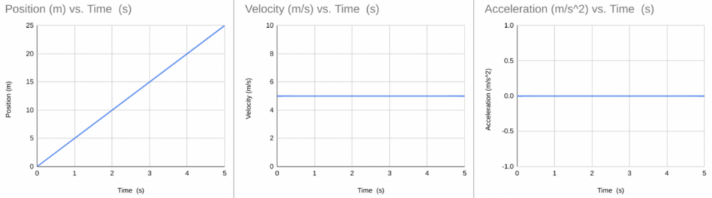
There are three types of motion graphs that you will come across in the average high school physics course – position vs time graphs, velocity vs time graphs, and acceleration vs time graphs. An example of each one can be seen below.

The position vs time graph (on the left) shows how far away something is relative to an observer.

The velocity vs time graph (in the middle) shows you how quickly something is moving, again relative to an observer.

Finally, the acceleration vs time graph (on the right) shows how quickly something is speeding up or slowing down, relative to an observer.

Because all of these are visual representations of a movement, it is important to know your frame of reference. We learned in our introduction to kinematics that two people can observe the same event but describe it differently depending upon where they stand. If this or anything about the position, velocity, and/or acceleration is still a bit confusing, revisit our kinematics post and our acceleration post before moving on.

Describing Motion with Position vs Time Graphs

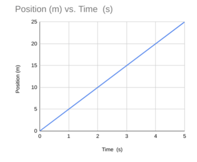
We typically start with position-time graphs when learning how to interpret motion graphs – generally because they’re the easiest to try to picture. Let’s look at the position vs time graph from above. We see that our vertical axis is Position (in meters) and that our horizontal axis is Time (in seconds). This means we know how far away an object has moved from our observer at any given time. This particular graph shows an object moving steadily away from our observer.

Position vs Time Graph for Multi-Stage Motion

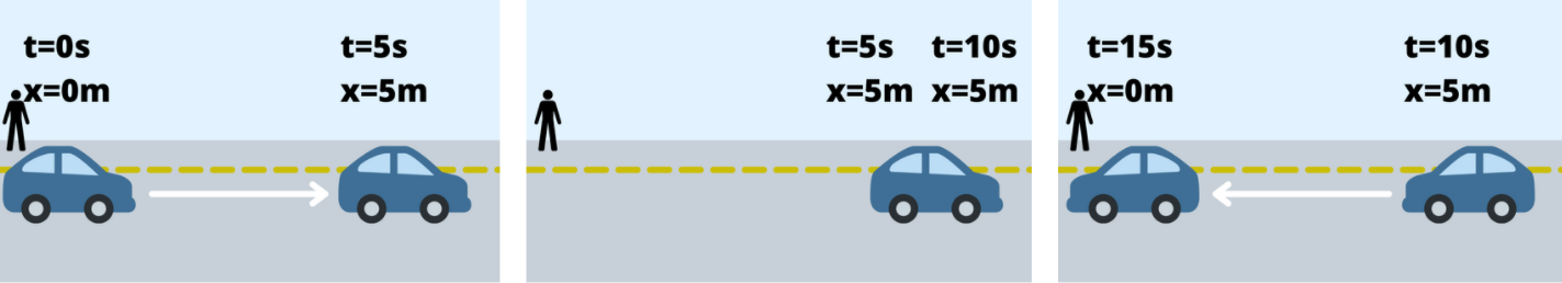
Let’s consider the graph and images below. We are still considering a position vs time graph, but this time we are looking at motion that changes. The car begins by moving 5 meters away from the observer in the first 5 seconds. After that, the car remains stopped 5 meters away from the observer for another 5 seconds. Finally, the car turns around and moves for 5 seconds back to its original position, 0 meters from the observer.

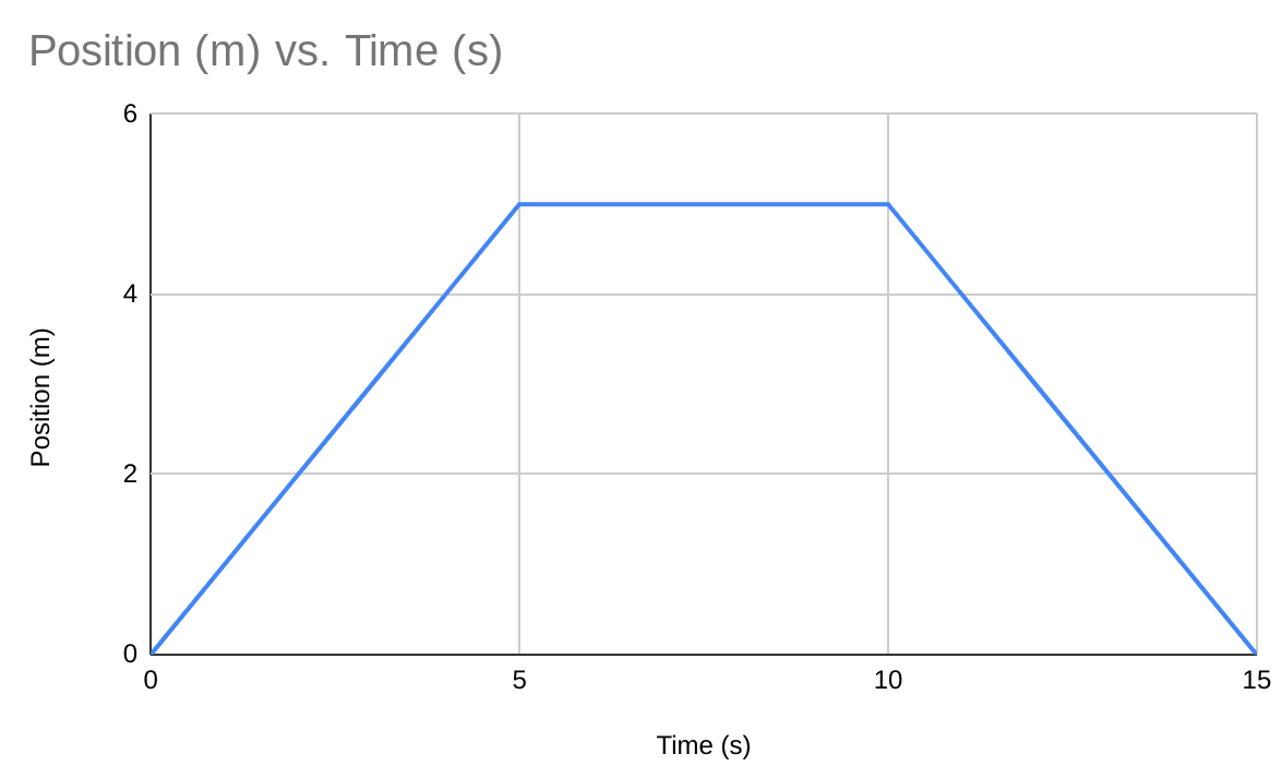
There are two key points that we can take from the example above. The first is that our position vs time graph shows how far away we are at any given time and nothing else. It cannot tell us distance or displacement – we would have to do a little mathematics to find those out. The second is that the change in position is not always positive. Here, we’ve defined moving to the right as positive. So, in the beginning, when the car was moving to the right, its position increased. In the end, when it moved back to the left, it was moving in the negative direction.

Position vs Time Graph for Passing an Observer

This implies that the position could, potentially, go below the x-axis. Let’s look at an example combining these two points in practice.

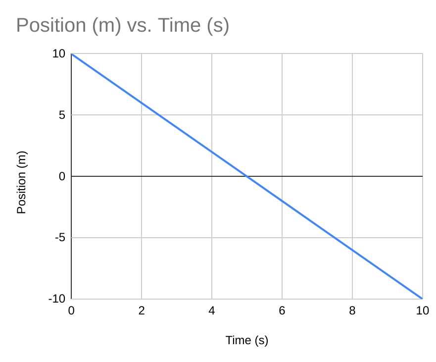
This time, our car started to the right, and drove straight past our observer to the left. At t=0\text{ s}, the car was 10\text{ m} to the right of our observer, so its position was x=10\text{ m}. As it passed the observer, its position was x=0\text{ m} at t=5\text{ s}. The car then ended its journey 10\text{ m} to our observers left at t=10\text{ s} so that its final position was x=-10\text{ m}.

Finding Distance and Displacement from a Position vs Time Graph

Example 1: Constant Position vs Time Graph

We’ll continue working from the graph above as we have already pulled the important values from it. Because we have a simple, straight line we only need the values from the very beginning and very end of the car’s journey, which we already pulled out above:

• t_{1}=0\text{ s}
• x_{1}=10\text{ m}
• t_{2}=10\text{ s}
• x_{2}=-10\text{ m}

Finding Distance From A Position-Time Graph

As we learned from our introduction to kinematics lesson, we know that the equation for distance is:

Formula for Distance d_{T}=d_{1}+d_{2}

The problem here is that we didn’t pull out any d values from our position vs time graph, only x values. We can still use those, though. In general, if you take the absolute value of an x value, it can be thought of as a d value and plugged into our distance equation. So the d values we’ll be using are:

• d_{1}=\lvert x_{1} \rvert =\lvert 10\text{ m} \rvert = 10\text{ m}
• d_{2}=\lvert x_{2} \rvert =\lvert -10\text{ m} \rvert = 10\text{ m}

Now we can plug these values into our equation and solve for our distance.

d_{T}=d_{1}+d_{2}=10\text{ m}+10\text{ m}=20\text{ m}

Finding Displacement From A Position vs Time Graph

Our equation for displacement is:

Formula for Displacement \Delta x=x_{f}-x_{i}

In this case, we will be using x_{2} as x_{f} and x_{1} as x_{i} as they represent the end and beginning of our movements, respectively. When we plug in our values, we find:

\Delta x=x_{2}-x_{1}=-10\text{ m}-(10\text{ m})=-20\text{ m}

In this case, the negative sign makes sense as our line is moving down the graph and the car moved from right to left, which we had previously defined as positive to negative.

Example 2: Changing Position vs Time Graph

Now that we know the basics of finding distance and displacement from a position vs time graph, let’s get a bit more in-depth. We’ll return to the graph about the car that moved forward, stopped, and then turned around and returned to its original position. The graph has been copied below for convenience.

How to Find Distance From A Position vs Time Graph

Finding distance from these graphs can get a bit complex as you’ll need to find several different values. If you’ll notice, the slope of our graph changes regularly – the line seems to turn. Each segment with a unique slope requires our attention. So, we’ll need to look at t=0\text{ s} through t=5\text{ s}, t=5\text{ s} through  t=10\text{ s}, and  t=10\text{ s} through  t=15\text{ s}.

We’ll want to look at the position value on the left and right of each side of those segments and find the absolute value of the delta between those values. These will serve as the d values that we will plug into our distance equation.

• d_{1}=\lvert 5\text{ m}-0\text{ m} \rvert =5\text{ m}
• d_{2}=\lvert 5\text{ m}-5\text{ m} \rvert =0\text{ m}
• d_{3}=\lvert 0\text{ m}-5\text{ m} \rvert =5\text{ m}

We can now plug all of these values into our equation and solve for distance.

d_{T}=d_{1}+d_{2}+d_{3}=5\text{ m}+0\text{ m}+5\text{ m}=10\text{ m}

How to Find Displacement From A Position vs Time Graph

Finding displacement from a graph that changes how it’s moving is a bit easier than finding the distance. Because displacement only concerns the distance between the starting and ending positions of an object’s motion, we only need to find the position at the rightmost point on the graph (t=15\text{ s}) and the leftmost point on the graph (t=0\text{ s}). The positions at these times will serve as our x_{f} and x_{i} values respectively. 

• x_{f}=0\text{ m}
• x_{i}=0\text{ m}

Now that we have these values, we can plug them into our displacement formula and solve:

\Delta x=x_{f}-x_{i}=0\text{ m}-0\text{ m}=0\text{ m}

Finding Velocity from a Position vs Time Graph

Now that we know how to find distance and displacement from a position vs time graph, we can start finding another value – velocity. If you think about it, these distances and displacements that we’re finding are occurring over some amount of time (as given by the graph) and all we really need to find velocity is displacement and time. So let’s start with a simple graph – the one of an object moving steadily away.

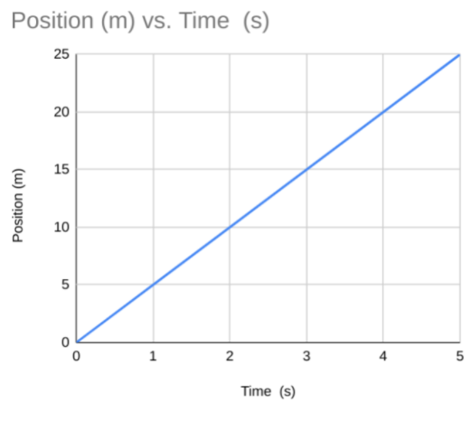
The displacement for the movement depicted by this graph would be \Delta x=25\text{ m}-0\text{ m}=25\text{ m} and because our time here moves from t=0\text{ s} to t=5\text{ s}, we have a change in time of \Delta t=5\text{ s}. This is enough information for us to solve for the velocity using the equation we learned before:

v=\dfrac{\Delta x}{\Delta t}=\dfrac{25\text{ m}}{5\text{ s}}=5\text{ m/s}

One very important thing you may notice if you’re savvy with slopes is that the slope of this graph is also equal to 5. (If you are not particularly savvy with slopes, I would recommend reviewing how to solve for slope as we’ll be relying on that knowledge for most of what remains of this post.) This similarity is no mere coincidence. The velocity of any movement will always be equal to the slope of the position-time graph at that time.

Proving Velocity is the Slope of Position vs Time Graphs

The slope of any given straight line can be found with the equation

Slope Formula m=\dfrac{y_{2}-y_{1}}{x_{2}-x_{1}}

Here, m is the slope, y_{2} and y_{1} are two different position values, and x_{2} and x_{1} are the time values corresponding to the two position values.

Let’s begin by selecting two points off of our graph above (being sure to include the units when we do). Let’s take (2\text{ s},10\text{ m}) and (4\text{ s},20\text{ m}) and plug the values in:

m=\dfrac{20\text{ m}-10\text{ m}}{4\text{ s}-2\text{ s}}

This setup of subtracting the rightmost value from the leftmost value should look a bit familiar. Another way to think of it is as taking a final value and subtracting an initial value, much like a delta. In fact, this is equivalent to a change in position over a change in time – the definition of velocity.

Let’s make sure our slope works out to be a velocity value before we jump to any conclusions, though. If the slope of this graph is also the velocity of the same motion, two things need to be true. First, we need a numerical value of 5. Second, we need our units to be in m/s. Let’s solve the equation above and see what we get.

m=\dfrac{20\text{ m}-10\text{ m}}{4\text{ s}-2\text{ s}}=\dfrac{10\text{ m}}{2\text{ s}}=5\text{ m/s}

We have a value that matches the velocity we solved for in both numerical value and physical units. We could have selected any two points on our graph and received the same result. The part of this that truly proves the slope of any position-time graph is the velocity is that the units of our slope work out to be m/s – the units for velocity.

Example 1: Finding Velocity from a Position vs Time Graph

Let’s try finding our velocity again, but using the slope formula. We’ll reuse the graph below that we saw earlier in this article.

We’ll want to begin by selecting the points we want to use. This graph is a straight line which means its slope never changes so it won’t particularly matter what two points we choose. Since we have a point where our x value is zero and a separate point where our y value is zero, we may as well use those to make the mathematics easier. So, the values we’ll be using here are:

• y_{2}=0\text{ m}
• y_{1}=10\text{ m}
• x_{2}=5\text{ s}
• x_{1}=0\text{ s}

Now, all we need to do is set our velocity equal to our slope, plug in our values, and solve for our velocity:

v=m=\dfrac{y_{2}-y_{1}}{x_{2}-x_{1}}=\dfrac{0\text{ m}-10\text{ m}}{5\text{ s}-0\text{ s}}=\dfrac{-10\text{ m}}{5\text{ s}}=-2\text{ m/s}

Here, we get a negative velocity of v=-2\text{ m/s}. If we look at our graph, we see it has a negative slope, so we should have expected this negative velocity from the start. If you ever get a positive when you expected a negative or vice versa, check to make sure you plugged your values into your formula in the correct order. That simple mistake has thrown many scientists off course.

Example 2: Finding Velocity with Changing Motion

Being able to find the velocity of a simple, straight position vs time graph is all well and good, but there will be times when you’ll have to split a graph apart. Let’s revisit the graph below as an example of this.

We already said before that we could split this graph up into a few different chunks based on when the slope changes. We know what happens when we have a positive slope and what happens when we have a negative slope, though, so let’s look at just the middle section where it’s flat. Here, the values we can pull from the line segment are:

• y_{2}=5\text{ m}
• y_{1}=5\text{ m}
• x_{2}=5\text{ s}
• x_{1}=10\text{ s}

If we plug these values into our slope formula, we can find that

v=m=\dfrac{y_{2}-y_{1}}{x_{2}-x_{1}}=\dfrac{5\text{ m}-5\text{ m}}{5\text{ s}-10\text{ s}}=\dfrac{0\text{ m}}{5\text{ s}}=0\text{ m/s}

Since the segment was a flat line with a slope of 0, the velocity also had to be 0\text{ m/s}. If we recall, this graph depicted a car that moved in the positive direction, stopped and remained motionless, and then moved back in the negative direction. The middle segment of this graph, the one that we looked at, corresponds to when the car was stopped so again. Therefore, it makes sense that we would see a velocity of 0\text{ m/s}.

Describing Motion with Velocity vs Time Graphs

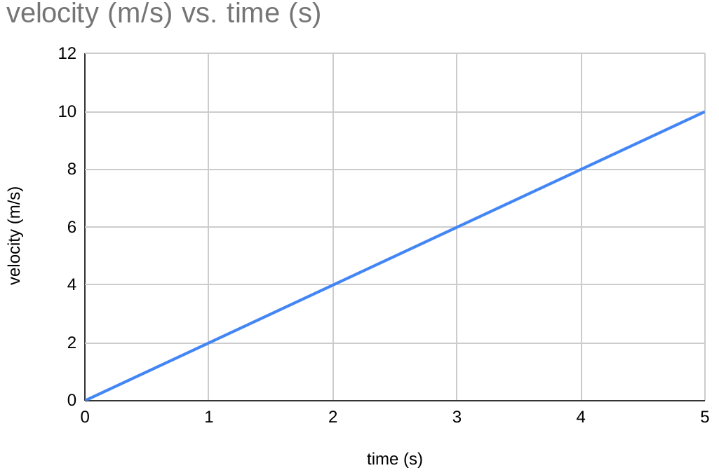
Velocity-time graphs are relatively similar to position-time graphs, and just as important in the study of motion graphs. We still have our time in seconds along the x-axis, but now we have our velocity in meters per second along the y-axis. Let’s consider the velocity-time graph below. 

To find the velocity of an object at any given time here, we simply need to read the value from the graph. There’s no mathematics to do or formulas to use. So, for example, at t=2\text{ s} the velocity is v=4\text{ m/s} because that is the value we read off of the graph. Similarly, the velocity is t=4\text{ s} is v=8\text{ m/s}. The fact that those two values differ and that the slope here is positive tells us that the motion in this graph is an object moving away from an observer and getting faster – like a car leaving a stoplight. We can also show more complicated motions and dip below the x-axis.

Velocity vs Time Graph with a Change in Direction

Let’s imagine a scenario for the graph to the right. We see that the graph starts with the object’s top velocity of v=10\text{ m/s} and then seems to get lower. The object reaches a velocity of v=0\text{ m/s} at t=2.5\text{ s}. While it may make sense to say that the object is now at the same point as the observer, we can’t actually infer that. All we can tell from here is that the object is momentarily at rest relative to the observer. The velocity then continues decreasing to v=-10\text{ m/s}, implying that the object is now moving in the negative direction. A real-life scenario for this may be that you observe someone pulling into a long driveway, stopping briefly at the end, and then backing down it.

Velocity vs Time Graph for Multi-Stage Motion

Now, let’s return to our car from before that moved in the positive direction, stopped, and then came back. Since the slope in each segment of the position graph was constant, we assumed that the car’s movements had a constant velocity and that it had zero velocity when it stopped. The velocity-time graph for this motion would look a bit like this:

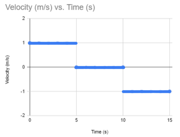
You can see that the velocity remains a constant v=1\text{ m/s} while the car moves to the right, changes to v=0\text{ m/s} while the car stops, and then becomes v=-1\text{ m/s} while the car moves back to the left. 

Finding Displacement from a Velocity vs Time Graph

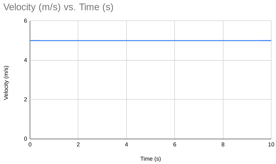
Much like how we could find a velocity from a position-time graph, we can find displacement from a velocity-time graph. This process will be a bit different. Instead of finding the slope of the velocity graph, we will be finding the area under the velocity graph. This may sound counterintuitive, but we can prove that it works by checking our units. Let’s say that an object moves at 5\text{ m/s} for 10\text{ s}. The velocity-time graph for this motion would look like this:

Proving Displacement is the Area under Velocity vs Time Graphs

To prove that the area under this velocity-time graph is the object’s displacement, let’s start with figuring out the displacement. The equation for displacement is \Delta x=vt. In this case, we know v=5\text{ m/s} and t=10\text{ s}. Therefore, \Delta x=(5\text{ m/s})\cdot (10\text{ s})=50\text{ m}.

Now that we know we’re looking for a displacement of 50\text{ m}, let’s try finding the area under the curve. Specifically, this is the area between the line of our graph and the x-axis. We’ll start by drawing a shape – in this case, a rectangle. We’ll also include values for its base and height.

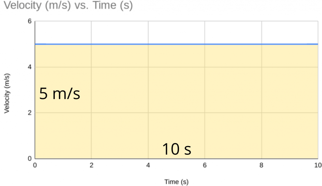
It’s worth noting here that the units along each axis were also included for the base and height of the rectangle. The equation for the area under the curve is the one you would use to find the area of a rectangle, A=bh. So, let’s pull down our values and solve our equation:

• b=10\text{ s}
• h=5\text{ m/s}

A=bh=(10\text{ s})\cdot (5\text{ m/s})=50\text{ m}

As a result, we obtained the same numerical value of 50, but more to the point we obtained the correct units. The area under the curve of a velocity graph will always be a displacement. Let’s look at a couple of more examples. If you’re uncertain about your ability to remember the equations for the area of a rectangle or triangle, it may be worth writing them in your notes or referencing a formula sheet such as this one.

Example 1: Finding Displacement for Multiple Velocities

The graph above was pretty simple, so let’s look at some more complex motion graphs. We can return to the velocity-time graph for our car that moved to the right, paused, then moved back to the left.

We already know that our displacement for this motion is 0\text{ m}. Let’s start by sectioning off our graph here into shapes we cam find the area of. Again, we’re looking for the area between the line of the graph and the x-axis.

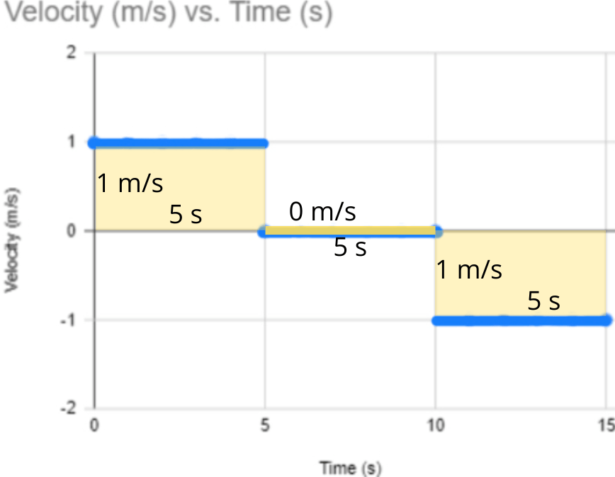
It seems strange to have a negative value for the height of a shape as you’ve likely been told that area should always be a positive value. We’ll see why having a negative height when the graph is below the x-axis is both allowed and important. Now that we have all of our rectangles we can start finding their area.

Let’s begin with the rectangle farthest to the left.

• b=5\text{ s}
• h=1\text{ m/s}

A_{left}=bh=(5\text{ s})\cdot (1\text{ m/s})=5\text{ m}

Now we can solve for the area of our middle rectangle. This may seem like a trick question as it is, essentially, just a flat line, but we’ll still want to include it.

• b=5\text{ s}
• h=0\text{ m/s}

A_{middle}=bh=(5\text{ s})\cdot (0\text{ m/s})=0\text{ m}

Finally, let’s find the area of the rectangle on the right. This has a negative value for its height so it should also have a negative area, strange as that may seem.

• b=5\text{ s}
• h=-1\text{ m/s}

A_{right}=bh=(5\text{ s})\cdot (-1\text{ m/s})=-5\text{ m}

Now that we know the area of all three rectangles, we’ll want to add those areas together to find the total area under the velocity-time curve and therefore also our total displacement.

\Delta x=A_{Total}=A_{left}+A_{middle}+A_{right}=5\text{ m}+0\text{ m}+(-5\text{ m})=0\text{ m}

Now, we see the expected value of 0\text{ m} that we’d found before. It’s important to note that this was only possible because one of our rectangles had a negative area.

Example 2: Finding Displacement with Changing Velocity

We know we can use rectangles to find the area under a velocity-time graph, but not all graphs are horizontal lines. Sometimes, graphs are diagonal which requires us to find the area of a different shape – a triangle. Consider the velocity-time graph.

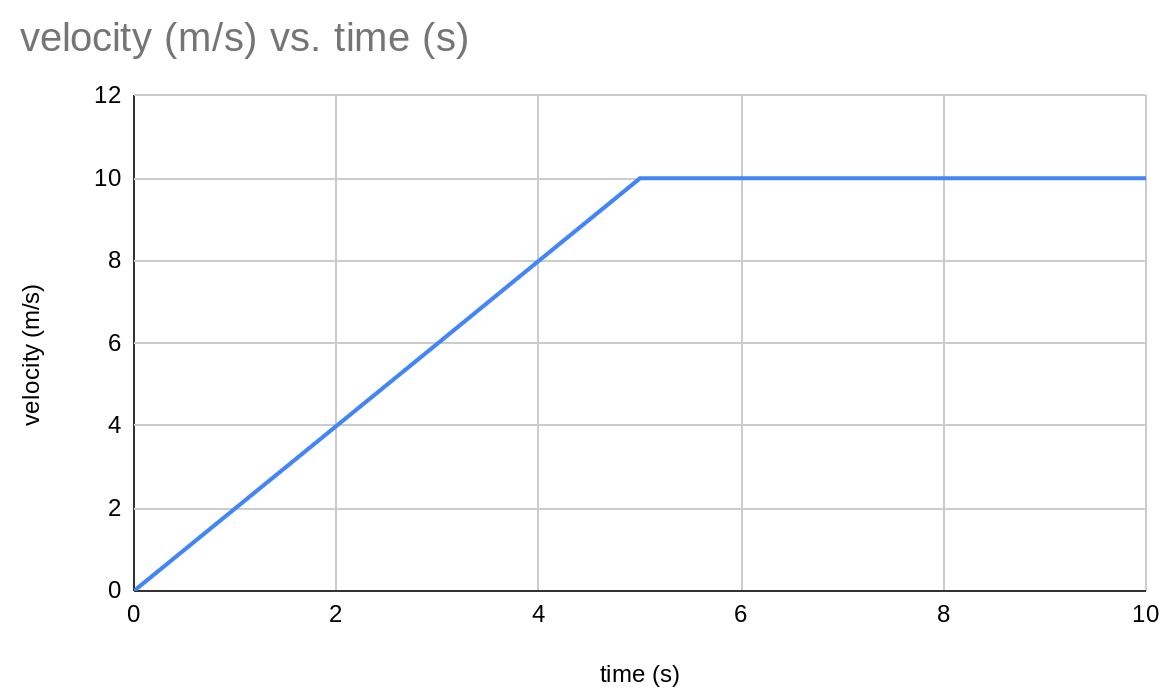
We can create a rectangle on the right where the velocity is constant, but the area where it’s increasing will not look like a rectangle at all. Instead, this is where we’ll have to create a section that is a triangle.

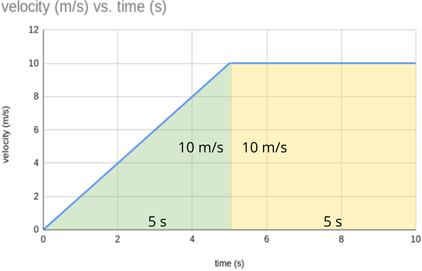
We now have two separate shapes. Much like when we had three separate rectangles, we’ll find the area of each shape individually and then add those two areas together to find the overall displacement for this motion. Let’s start with the triangle.

• b=5\text{ s}
• h=10\text{ m/s}

A_{Triangle}=\dfrac{1}{2}bh=\dfrac{1}{2}(5\text{ s})\cdot (10\text{ m/s})=25\text{ m}

Now, we can find the area of the rectangle portion.

• b=5\text{ s}
• h=10\text{ m/s}

A_{Rectangle}=bh=(5\text{ s})\cdot (10\text{ m/s})=50\text{ m}

Finally, we’ll add these two values to find our total displacement:

\Delta x=A_{Total}=A_{Triangle}+A_{Rectangle}=25\text{ m}+50\text{ m}=75\text{ m}

Finding Acceleration from a Velocity vs Time Graph

At this point, it may not shock you to learn that the slope of a velocity-time graph can tell us just as much as the area under its curve. Instead of displacement, though, the slope of a velocity graph will tell us an object’s acceleration. Let’s consider the graph.

The velocity of the object being shown in this graph is steadily increasing by 2\text{ m/s} every 1\text{ s}. With that information, we can prove that a=\Delta v/\Delta t=(2\text{ m/s})/(1\text{ s})=2\text{ m/s}^2. Now that we know what our acceleration should be, let’s try to find it by finding the slope of the velocity time graph.

Proving Acceleration is the Slope of Velocity vs Time Graphs

If you remember from earlier, the slope of any given straight line can be found with the equation:

Slope Formula m=\dfrac{y_{2}-y_{1}}{x_{2}-x_{1}}

Let’s begin by selecting two points off of our graph above (being sure to include the units when we do). Let’s take (2\text{ s},4\text{ m/s}) and (4\text{ s},8\text{ m/s}) and plug the values in.

m=\dfrac{8\text{ m/s}-4\text{ m/s}}{4\text{ s}-2\text{ s}}

Again, this should look like a set of delta values – change in velocity over change in time, specifically. This is the definition of acceleration. While you may already be able to see how this will turn into proof that acceleration is the slope of a velocity graph, let’s keep going. What we’ll be looking for when we solve this equation this time will be a numerical value of 2 and units of m/s².

m=\dfrac{8\text{ m/s}-4\text{ m/s}}{4\text{ s}-2\text{ s}}=\dfrac{4\text{ m/s}}{2\text{ s}}=2\text{ m/s}^2

Notice that we have a value that matches the acceleration we solved for before. We could have selected any two points on our graph and received the same result. The part of this that truly proves the slope of any velocity-time graph is the acceleration is that the units of our slope work out to be m/s² – the units for acceleration.

Example 1: Finding Negative Acceleration

Let’s consider the velocity vs time graph.

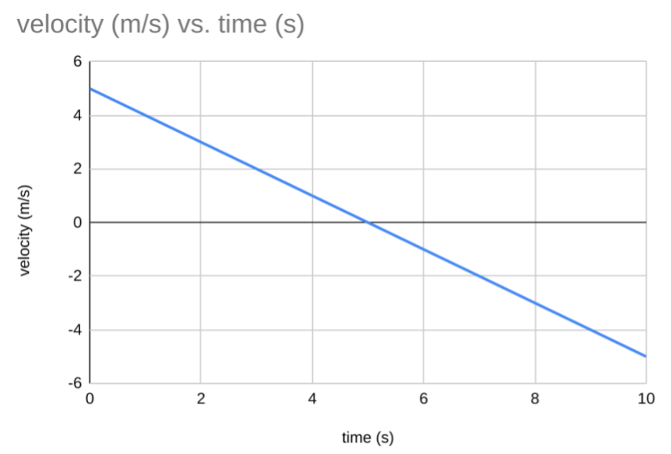
We can see that the graph has a constant, negative slope so we can choose any two points we want and we should get the correct acceleration, which should also be a negative value. Whenever possible, it’s worth choosing values with zeros, so let’s select the points (0\text{ s},5\text{ m/s}) and (5\text{ s},0\text{ m/s}). Now that we have our points, let’s pull out the values we need and plug them into our slope formula to solve for the acceleration of this object.

• y_{2}=0\text{ m/s}
• y_{1}=5\text{ m/s}
• x_{2}=5\text{ s}
• x_{1}=0\text{ s}

If we plug these values into our slope formula, we can find that

a=m=\dfrac{y_{2}-y_{1}}{x_{2}-x_{1}}=\dfrac{0\text{ m/s}-5\text{ m/s}}{5\text{ s}-0\text{ s}}=\dfrac{-5\text{ m/s}}{5\text{ s}}=-1\text{ m/s}^2

Example 2: Finding Multiple Accelerations

Let’s consider a more complex example with the velocity-time graph below.

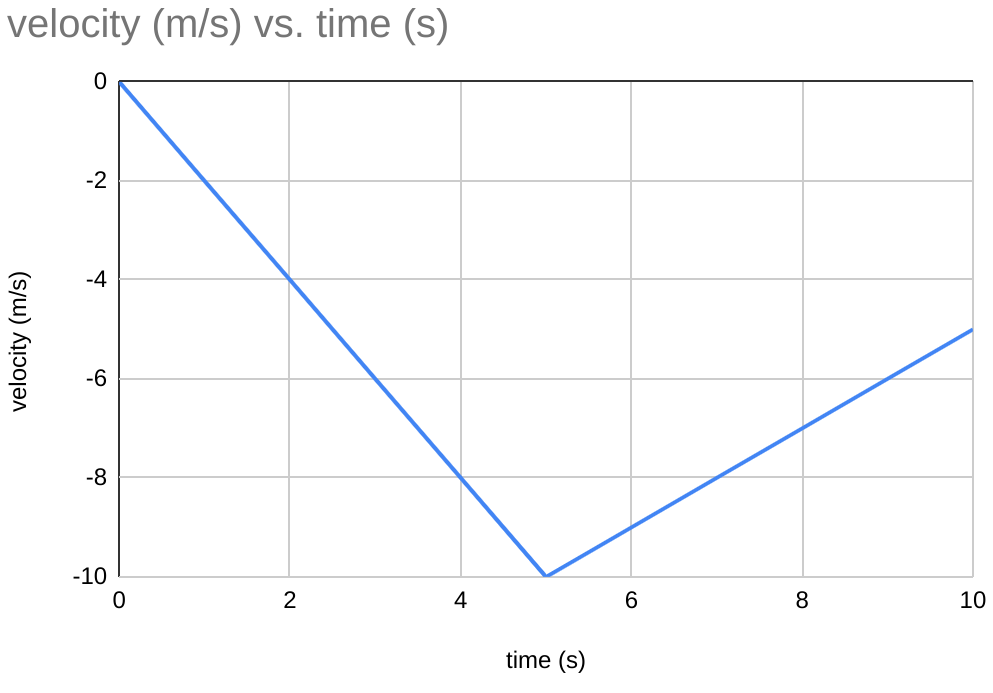
This graph has a change in its slope. This means we have two separate sections that we can look at: before t=5\text{ s} and after t=5\text{ s}.

Let’s consider the after t=5\text{ s} portion of the graph. Assuming that our acceleration will be negative because our velocity values are always negative is a common mistake among budding physicists. We’ll see here that this isn’t always true. Let’s choose the points (5\text{ s},-10\text{ m/s}) and (10\text{ s},-5\text{ m/s}) and plug these values into our slope formula.

• y_{2}=-5\text{ m/s}
• y_{1}=-10\text{ m/s}
• x_{2}=10\text{ s}
• x_{1}=5\text{ s}

If we plug these values into our slope formula, we can find that:

a=m=\dfrac{y_{2}-y_{1}}{x_{2}-x_{1}}=\dfrac{-5\text{ m/s}-10\text{ m/s}}{10\text{ s}-5\text{ s}}=\dfrac{5\text{ m/s}}{5\text{ s}}=1\text{ m/s}^2

We see that even though our velocity values are negative, our slope is still positive so our acceleration must still be positive. Be careful when looking at motion graphs and making early assumptions. Things are sometimes more complicated than they appear.

Describing Motion with Acceleration vs Time Graphs

Last but not least, we can describe an object’s motion with an acceleration vs time graph. These will likely be graphs with zero slope while you are starting your study of motion graphs. You may find them becoming more complicated if you pursue a career in physics, but for now, we can keep things simple. The below graph is a standard example of an acceleration graph you may see.

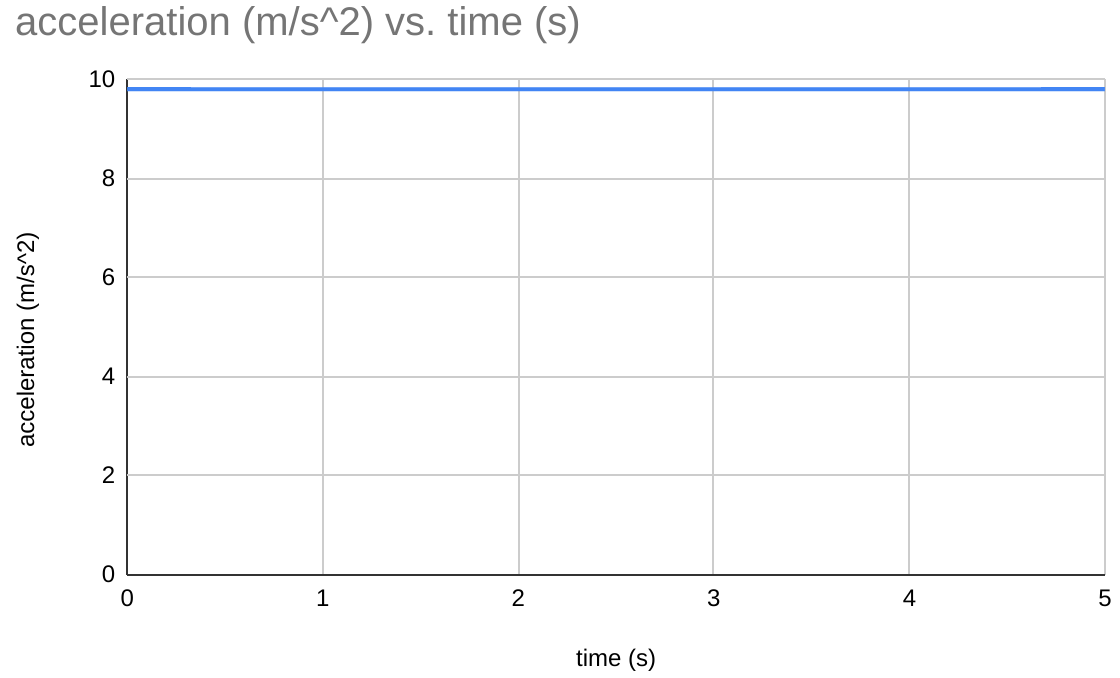
This graph actually shows acceleration due to gravity on Earth’s surface at a constant value of 9.81\text{ m/s}^2. The other acceleration-time graph you’re likely to see in a high school physics class may look more like this:

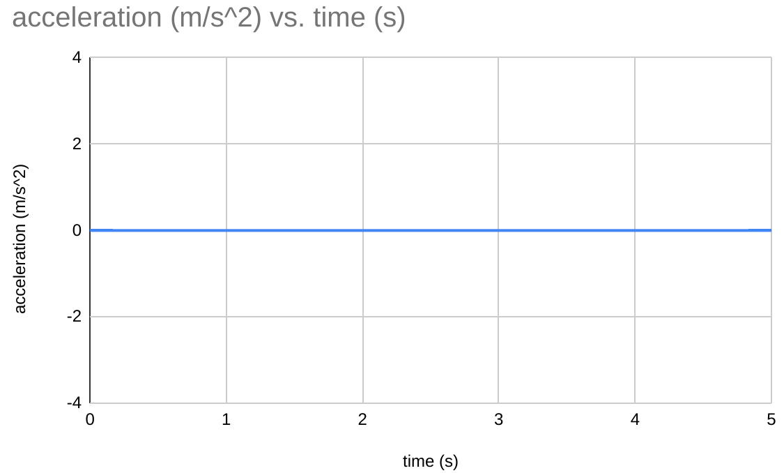
This would indicate that the object’s velocity is not changing, or perhaps that it isn’t moving at all. 

It is worth noting that the area under the curve of an acceleration vs time graph is equal to an object’s velocity, much like how the area under a velocity vs time graph is the displacement. Most high school physics classes won’t spend much time on this idea, but as you progress through your physics career this idea may come up. If you’d like to prove it to yourself, you could follow the same proof we used when proving the relationship between a velocity-time graph and an object’s displacement.

Pairing Motion Graphs

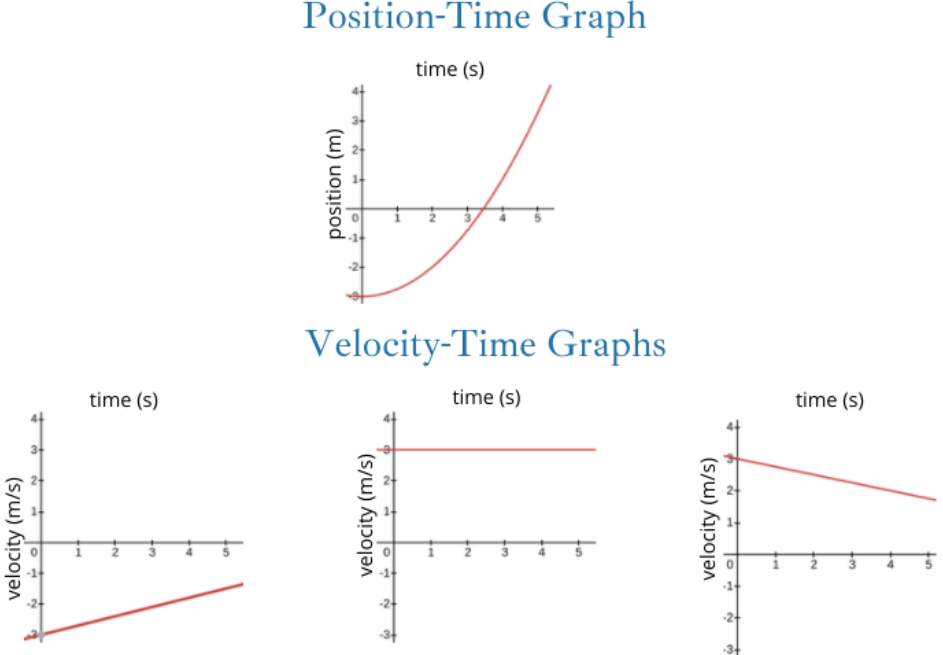
The last skill we’ll cover for motion graphs is determining which pair of graphs represent the same motion. We can make more than one graph to describe any given motion. For example, we had both a position-time graph and a velocity-time graph for our car moving to the right, pausing, and then coming back to the left. We can extend this idea to include acceleration graphs too. Let’s consider the three graphs you were presented with at the beginning of this article.

We can see the position vs time graph on the left has a constant, positive slope. Since we know that velocity is the slope of a position vs time graph, our velocity must therefore be a constant, positive value. Indeed, we see that the velocity vs time graph here is constantly at 5\text{ m/s}. If we continue following this logic, we can assume that our acceleration should be zero as the slope of our velocity vs time graph is zero. And, again, we see that this holds true as the acceleration vs time graph is constant at 0\text{ m/s}^2.

While it may be easy to see that these three motion graphs are connected after looking at them for a few moments, you’ll want to be able to compare more complex graphs throughout your physics career. There are a few steps you can take to achieve this goal.

The Steps to Pairing Motion Graphs

Step 1: Observe the Shape and Make a Prediction

Odds are, you’ll see three different shapes when looking at position graphs, three shapes when looking at velocity graphs, and only two shapes when looking at acceleration graphs. Without even looking at the numbers on these graphs, the shapes can tell you a lot. Here are the shapes of each graph you may see throughout your high school physics career:

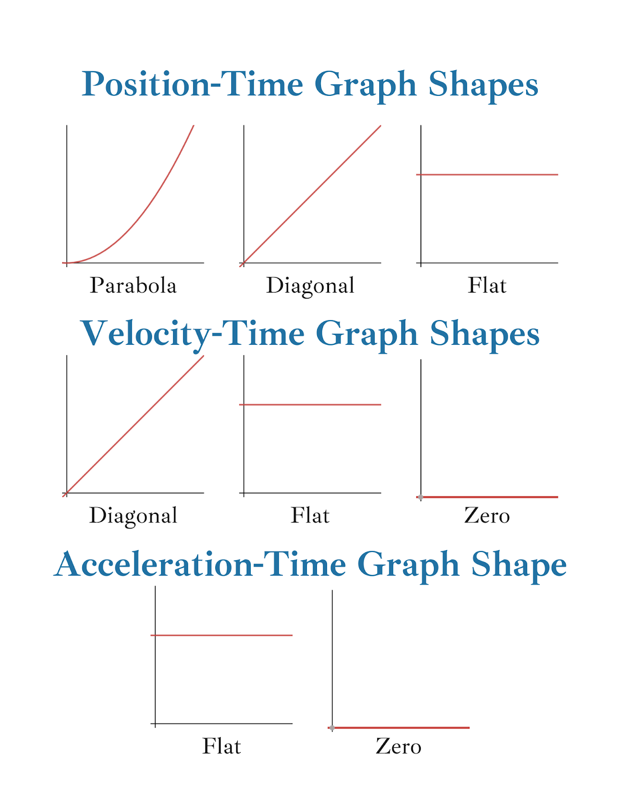
All of these examples are of positive values but know that they may be flipped. This would simply mean that the slope values are negative instead of positive. Just from glancing at the graphs above, even though they don’t have any number, you could match them up just by looking at the slopes.

Corresponding Shapes on Motion Graphs

Here’s a chart of how the different shapes match up.

Position-Time Graphs		Velocity-Time Graphs		Acceleration-Time Graphs
Parabola	↔	Diagonal	↔	Flat
Diagonal	↔	Flat	↔	Zero
Flat	↔	Zero	↔	Zero

You may notice that the arrows here go both ways and for good reason. While you’ll need to do some math to know exactly which parabola-shaped position-time graph matches a diagonal-shaped velocity-time graph, those two shapes will always go together, regardless of which you start with.

Step 2: Decide if it is Positive or Negative

There is one more step you can take in matching up motion graphs before you start doing any actual math, which is looking for positive or negative slopes. Let’s look at this position-time graph.

We can see that the slope here is negative. The curve is above the x-axis so the values are positive, but the slope itself is negative. We know that this shape of the position-time graph will go with a flat velocity-time graph, but we need to pick the right one. We may need some mathematics for this, but let’s first try to narrow down our options. Let’s say you had to pick between the three velocity-time graphs below.

We’ve decided that our graph should be a straight, horizontal line. All three of these graphs match that description. We also said that our slope is negative, and only two of the velocity-time graphs have negative values. So, without doing any mathematics, we know that the positive-time graph above will have to be paired with the middle velocity-time graph or the right velocity-time graph. To find out for sure, we’ll have to add some numbers and do some math.

Step 3: Calculate the Slope and Compare

Let’s take that same position-time graph and the two velocity-time graphs we couldn’t decide between. As you’ll see, they now have some numbers so that we can do some math to actually match the correct graphs.

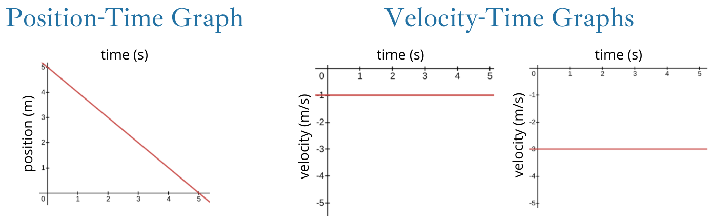
We’ll need to begin by finding the slope of the position-time graph. To keep things simple, let’s use (0\text{ s},5\text{ m}) and (5\text{ s},0\text{ m}). Now let’s pull out some values and solve for slope.

• y_{2}=0\text{ m}
• y_{1}=5\text{ m}
• x_{2}=5\text{ s}
• x_{1}=0\text{ s}

m=\dfrac{y_{2}-y_{1}}{x_{2}-x_{1}}=\dfrac{0\text{ m}-5\text{ m}}{5\text{ s}-0\text{ s}}=\dfrac{-5\text{ m}}{5\text{ s}}=-1\text{ m/s}

So, the velocity-time graph that matches our position-time graph here should have a value of -1\text{ m/s}. If we look, the velocity-time graph on the left has its line moving through -1\text{ m/s} so that must be the correct velocity-time graph.

We used these three steps of looking at the shape, looking at positive or negative, and then calculating the slope to go from a position-time graph to a velocity-time graph, but they can help us do much more than that. They can help us match up all three kinds of graphs or any pair of motion graphs – even a position-time graph and an acceleration-time graph.

Example 1: Which Pair of Graphs Represent the Same Motion?

Let’s consider the position-time graph below and try to match it to the correct velocity vs time graph.

Observe the Shape

Right off the bat, we know we have a parabola-shaped position-time graph. From that, we can narrow down our velocity-time graph options. A parabola position-time graph always goes to a diagonal velocity-time graph so we can cross off the middle graph immediately. Now we’re left with two different choices.

You may think you have the right answer already (and indeed you might), but let’s think through this carefully. We already matched up our shapes so now it’s time to compare our positives and negatives.

Decide if it is Positive or Negative

The parabola in the position-time graph points upward so it has a positive slope. That means our velocity-time graph needs to be positive. If you’re thinking too carefully about slope, you may be drawn to the graph on the left. While it’s true that the graph on the left has a positive slope, it actually contains negative values. The values are what’s important here, not the slope. Instead, the graph on the right is the correct choice here. We knew we needed a diagonal velocity-time graph with positive values and we only had one option. You may often encounter examples like this, but be careful to always check your instincts before answering too quickly.

It is also worth noting here that a helpful trick for recognizing whether a velocity-time graph could give a positive slope to a position-time graph is if the curve of the velocity-time graph is over the x-axis. The same is true in reverse; a velocity-time graph with a curve below the x-axis will match with a position-time graph with a negative slope.

Example 2: Match the Velocity-Time Graph

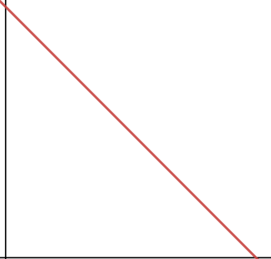
The same principles that we just used above can also help us transition from a velocity-time graph to an acceleration-time graph. Let’s consider the set of motion graphs below.

Observe the Shape

From the start, we can see that we have a diagonal-shaped velocity-time graph so we can eliminate our middle acceleration-time graph. Although we will want a flat graph, the middle one is on the x-axis, which would imply that our velocity-time graph has zero slope. If that were the case, it would be flat instead of diagonal.

Decide if it is Positive or Negative

Now that we are again down to two graphs, let’s look at the positives and negatives. The velocity-time graph has a negative slope so we’ll want an acceleration-time graph with a curve below the x-axis. This leaves us with only one option – the graph on the right. 

Again, we didn’t need to get to the mathematics. You could check the values if you wanted to, but often looking just at the shapes of your graphs will be enough. Just make sure you always think through both the shape of your motion graphs and if your positives and negatives line up.

Conclusion

Physicists use motion graphs to visualize data all the time. While the different types and shapes may be confusing at first, getting comfortable with them will help you make connections between the kinematics terms you’ve learned so far. It can also help you simplify problems by being able to visualize what the problem is asking you in a different way. If you take the time to get comfortable reading each time of motion graph, deriving different values from them, and matching them up, you’ll be well on your way to visualizing data the way research scientists do every day.