Synchronization Phenomena

Abstract

Complex systems are based on interacting local computational units may show non-trivial emerging behaviors. Examples are the time evolution of an infectious disease in a certain city that is mutually influenced by an ongoing outbreak of the same disease in another city, or the case of a neuron firing spontaneously while processing the effects of afferent axon potentials.

A fundamental question is whether the time evolutions of interacting local units remain dynamically independent of each other, or whether they will change their states simultaneously, following identical rhythms. This is the notion of synchronization, which we will study throughout this chapter. Starting with the paradigmatic Kuramoto model we will learn that synchronization processes may be driven either by averaging dynamical variables, or through causal mutual influences. On the way, we will visit piecewise linear dynamical systems and the reference model for infectious diseases, the SIRS model.

Complex systems are based on interacting local computational units may show non-trivial emerging behaviors. Examples are the time evolution of an infectious disease in a certain city that is mutually influenced by an ongoing outbreak of the same disease in another city, or the case of a neuron firing spontaneously while processing the effects of afferent axon potentials.

A fundamental question is whether the time evolutions of interacting local units remain dynamically independent of each other, or whether they will change their states simultaneously, following identical rhythms. This is the notion of synchronization, which we will study throughout this chapter. Starting with the paradigmatic Kuramoto model we will learn that synchronization processes may be driven either by averaging dynamical variables, or through causal mutual influences. On the way, we will visit piecewise linear dynamical systems and the reference model for infectious diseases, the SIRS model.

9.1 Frequency Locking

In this chapter, we will be dealing mostly with autonomous dynamical systems that may synchronize spontaneously. A dynamical system can also be driven by outside influences, being forced to follow the external signal synchronously.

Driven Harmonic Oscillator

For a start, we recapitulate the dynamical states of the driven harmonic oscillator,

$$\displaystyle \begin{aligned} \ddot x + \gamma\, \dot x + \omega_0^2\,x = F\left(\mathrm{e}^{i\omega t}+c.c.\right), \qquad \quad \gamma > 0\,, {} \end{aligned} $$

(9.1)

where ‘c.c.’ stands for conjugate complex. Of relevance will be the relation between the eigenfrequency $\omega _0$, damping $\gamma$, and the driving frequency $\omega$. In the absence of an external forcing, $F\equiv 0$, the solution is

$$\displaystyle \begin{aligned} x(t) \sim \mathrm{e}^{\lambda t} , \qquad \quad \lambda_{\,\,\,\,\pm} = -\frac{\gamma}{2} \pm \frac{1}{2}\,\sqrt{\gamma^2-4\omega_0^2}\,, {} \end{aligned} $$

(9.2)

which is damped/critical/overdamped for $\gamma <2\omega _0$, $\gamma =2\omega _0$ and $\gamma >2\omega _0$.

Frequency Locking

In the limit of long times, $t\to \infty$, the dynamics of the system follows the external driving. Due to the damping $\gamma >0$, this holds for all $F\ne 0$. For the ansatz

$$\displaystyle \begin{aligned} x(t) = a\mathrm{e}^{i\omega t}+c.c.\,, {} \end{aligned} $$

(9.3)

the amplitude a may contain, as a matter of principle,¹ an additional time-independent phase. Applying to (9.1) yields

$$\displaystyle \begin{aligned} \begin{array}{rcl} F & =&\displaystyle a\left(-\omega^2+i\omega\gamma+\omega_0^2\right) = -a\left(\omega^2-i\omega\gamma-\omega_0^2\right) \\[0.5ex] & =&\displaystyle -a\left(\omega+i\lambda_+\right) \left(\omega+i\lambda_-\right)\,, \end{array} \end{aligned} $$

where the eigenfrequencies $\lambda _{\pm }$ are given by (9.2). The solution for the amplitude a can then be written in terms of $\lambda _{\pm }$ or alternatively as

$$\displaystyle \begin{aligned} a = \frac{-F}{\left(\omega^2 -\omega_0^2\right) -i\omega\gamma}\,. {} \end{aligned} $$

(9.4)

The response becomes divergent, viz $a\to \infty$, at resonance $\omega =\omega _0$ and small dampings $\gamma \to 0$.

General Solution

The driven, damped harmonic oscillator (9.1) is an inhomogeneous linear differential equation. The general solution is hence given by the superposition of the special solution (9.4) with the general solution of the homogeneous system (9.2). The latter dies out for $t\to \infty$ and the system synchronizes with the external driving frequency $\omega$.

9.2 Coupled Oscillators and the Kuramoto Model

Whenever their dynamical behaviors are similar and the mutual couplings substantial, sets of local dynamical systems may synchronize. It is not necessary that the individual units show periodic dynamics on their own, coupled chaotic attractors can also synchronize. We start by discussing the simplest non-trivial set-up, the case of harmonically coupled uniform oscillators.

Limit Cycles

In suitable coordinates, free rotations such as

$$\displaystyle \begin{aligned} \mathbf{x}(t) = r\big(\cos{}(\theta(t)),\sin{}(\theta(t))\big), \qquad \theta(t) = \omega t+\theta_0, \qquad \dot\theta = \omega\,, \end{aligned}$$

describe periodic attractors, viz limit cycles. In the following we take the radius r as given, using the phase variable $\theta =\theta (t)$ for an effective description.

Coupled Dynamical Systems

We study the behavior of a collection of individual dynamical systems $i=1,\dots ,N$, each characterized by a limit cycle with natural frequency $\omega _i$. The coupled system obeys

$$\displaystyle \begin{aligned} \dot\theta_i = \omega_i + \sum_{j=1}^N\, \varGamma_{ij}(\theta_i,\theta_j), \qquad \quad i=1,\dots,N\,, {} \end{aligned} $$

(9.5)

where $\varGamma _{ij}$ are suitable coupling constants.

Kuramoto Model

A particularly tractable choice for the coupling constants $\varGamma _{ij}$ has been proposed by Kuramoto:

$$\displaystyle \begin{aligned} \varGamma_{ij}(\theta_i,\theta_j) = \frac{K}{N}\, \sin{}(\theta_j-\theta_i)\,, {} \end{aligned} $$

(9.6)

where $K\ge 0$ is the coupling strength. The factor $1/N$ ensures that the model is well behaved in the limit $N\to \infty$.

Two Coupled Oscillators

We consider first the case $N=2$,

$$\displaystyle \begin{aligned} \dot \theta_1 = \omega_1 + \frac{K}{2}\, \sin{}(\theta_2-\theta_1), \quad \quad \dot \theta_2 = \omega_2 + \frac{K}{2}\, \sin{}(\theta_1-\theta_2)\,, {} \end{aligned} $$

(9.7)

or

$$\displaystyle \begin{aligned} \varDelta\dot\theta = \varDelta\omega - K\, \sin{}(\varDelta\theta), \qquad \varDelta\theta = \theta_2-\theta_1, \qquad \varDelta\omega = \omega_2-\omega_1\,. {} \end{aligned} $$

(9.8)

The system has a fixpoint $\varDelta \theta ^*$ with regard to the relative phase, determined by

$$\displaystyle \begin{aligned} \frac{d}{dt}\varDelta\theta^* = 0, \qquad \quad \sin{}(\varDelta\theta^*) = \frac{\varDelta\omega}{K}\,, {} \end{aligned} $$

(9.9)

which leads to

$$\displaystyle \begin{aligned} \varDelta\theta^*\in[-\pi/2,\pi/2], \qquad \quad K > |\varDelta\omega|\,. {} \end{aligned} $$

(9.10)

This condition is valid for attractive coupling constants $K>0$. For repulsive $K<0$ anti-phase states are stabilized. We analyze the stability of the fixpoint using $\varDelta \theta =\varDelta \theta ^*+\delta$ and (9.8), obtaining

$$\displaystyle \begin{aligned} \frac{d}{dt}\delta = -\left(K\cos\varDelta\theta^*\right)\delta, \qquad \qquad \delta(t) = \delta_0\,\mathrm{e}^{-K\cos\varDelta\theta^* t}\,. \end{aligned}$$

The fixpoint is stable since $K\!>\!0$ and $\cos \varDelta \theta ^*\!>\!0$, due to (9.10). Consequently, a bifurcation is present.

• For $K<|\varDelta \omega |$ there is no phase coherence between the two oscillators, which are drifting with respect to each other.

• For $K>|\varDelta \omega |$ phase locking is observed, which means that the two oscillators rotate together with a constant phase difference.

The situation is illustrated in Fig. 9.1.

Fig. 9.1

The relative phase $\varDelta \theta (t)$ of two coupled oscillators, obeying (9.8), with $\varDelta \omega =1$ and a critical coupling strength $K_c=1$. For an undercritical coupling, $K=0.9$, the relative phase increases steadily, for an overcritical coupling $K=1.01$ it locks

Natural Frequency Distribution

We now examine what happens if we have a larger number of coupled oscillators, $N\to \infty$. We select the probability distribution $g(\omega )$ of the natural frequencies $\omega _i$, to be symmetric,

$$\displaystyle \begin{aligned} g(\omega) = g(-\omega), \qquad \qquad \int_{-\infty}^{\infty} g(\omega)\,d\omega = 1\,, {} \end{aligned} $$

(9.11)

The choice of a zero average frequency,

$$\displaystyle \begin{aligned} \int_{-\infty}^{\infty} \omega\, g(\omega)\,d\omega = 0\,, \end{aligned}$$

implicit in (9.11) is generally possible, as the dynamical equations (9.5) and (9.6) are invariant under a global translation

$$\displaystyle \begin{aligned} \omega \to \omega+\varOmega, \qquad \quad \theta_i \to \theta_i+\varOmega t\,, \end{aligned}$$

with $\varOmega$ being the initial non-zero mean frequency.

Order Parameter

The complex order parameter

$$\displaystyle \begin{aligned} r\,\mathrm{e}^{i\psi} = \frac{1}{N}\sum_{j=1}^N\, \mathrm{e}^{i\theta_j} {} \end{aligned} $$

(9.12)

is a macroscopic quantity that can be interpreted as the collective rhythm produced by the assembly of the interacting oscillating systems. The radius $r(t)$ measures the degree of phase coherence, with $\psi (t)$ corresponding to the average phase.

Molecular Field Representation

We rewrite the order parameter defined in (9.12) as

$$\displaystyle \begin{aligned} r\,\mathrm{e}^{i(\psi-\theta_i)} = \frac{1}{N}\sum_{j=1}^N\, \mathrm{e}^{i(\theta_j-\theta_i)}, \qquad \quad r\sin{}(\psi-\theta_i) = \frac{1}{N}\sum_{j=1}^N\, \sin{}(\theta_j-\theta_i)\,, \end{aligned}$$

retaining in the second step the imaginary component. Inserting the second expression into the governing equation (9.5), we find

$$\displaystyle \begin{aligned} \dot \theta_i = \omega_i + \frac{K}{N} \sum_j\,\sin{}(\theta_j-\theta_i) = \omega_i + Kr\sin{}(\psi-\theta_i)\,. {} \end{aligned} $$

(9.13)

The motion of individual oscillators $i=1,\ldots ,N$ is coupled to the other oscillators exclusively through the mean-field phase $\psi$, with a coupling strength that is proportional to the mean-field amplitude r.

The individual phases $\theta _i$ are drawn towards the self-consistently determined mean phase $\psi$, as can be seen in the numerical simulations presented in Fig. 9.2. Mean-field theory is exact for the Kuramoto model. It is nevertheless non-trivial to solve, as the self-consistency condition (9.12) needs to be fulfilled.

Fig. 9.2

Spontaneous synchronization in a network of limit cycle oscillators with distributed individual frequencies. Color coding with slowest–fastest (red–violet) natural frequencies. With respect to (9.5), an additional distribution of individual radii $r_i(t)$ has been assumed. These are slowly relaxing. Also shown is the mean field $r\mathrm {e}^{i\psi }= \sum _i r_i \mathrm {e}^{i\theta _i}/N$ (asterix), compare (9.12). Reprinted from Strogatz (2001) with permissions, Ⓒ 2001 Macmillan Magazines Ltd

Rotating Frame of Reference

The order parameter $r\mathrm {e}^{i\psi }$ performs a free rotation for long times $t\to \infty$ in the thermodynamic limit. With

$$\displaystyle \begin{aligned} r(t) \to r, \qquad \quad \psi(t) \to \varOmega t, \qquad \quad N \to \infty\,, \end{aligned}$$

and one can transform via

$$\displaystyle \begin{aligned} \theta_i \to \theta_i+\psi = \theta_i+\varOmega t, \qquad \quad \dot\theta_i \to \theta_i+\varOmega, \qquad \quad \omega_i \to \omega_i+\varOmega \end{aligned}$$

to the rotating frame of reference. The governing equation (9.13) then becomes

$$\displaystyle \begin{aligned} \dot \theta_i = \omega_i - Kr\sin{}(\theta_i)\,. {} \end{aligned} $$

(9.14)

This expression is identical to the one for the case of two coupled oscillators, see (9.8), when substituting Kr by K. It then follows directly that $\omega _i=Kr$ constitutes a special point.

Drifting and Locked Components

Eq. (9.14) has a fixpoint $\theta _i^*$ for which $\dot \theta _i=0$, as determined by

$$\displaystyle \begin{aligned} Kr\sin{}(\theta_i^*) = \omega_i, \qquad \quad |\omega_i| < Kr, \qquad \quad \theta_i^*\in\left[-\frac{\pi}{2},\frac{\pi}{2}\right]\,. {} \end{aligned} $$

(9.15)

The interval for $\theta _i^*$ is selected such that $\sin {}(\theta _i^*)\in [-1,1]$.

• Locked Units

  As we are working in the rotating frame of reference, $\dot \theta _i=0$ means that the participating limit cycles oscillate for $|\omega _i| < Kr$ with the average frequency $\psi$, they are “locked” to $\psi$.

• Drifting Units

  For $|\omega _i| > Kr$, the participating limit cycle drifts, i.e. $\dot \theta _i$ never vanishes. They do, however, slow down when they approach the locked oscillators, compare (9.14).

The distinct dynamics of locked and drifting units is illustrated in Figs. 9.1, 9.2, and 9.3.

Fig. 9.3

The region of locked and drifting natural frequencies $\omega$ within the Kuramoto model

Stationary Frequency Distribution

We denote with

$$\displaystyle \begin{aligned} \rho(\theta,\omega)\,d\theta \end{aligned}$$

the fraction of oscillators with natural frequency $\omega$ that lie between $\theta$ and $\theta +d\theta$. Of relevance for the following will be the continuity equation for $\rho =\rho (\theta ,\omega )$,

$$\displaystyle \begin{aligned} \frac{\partial\rho}{\partial t} + \frac{\partial}{\partial\theta}\Big(\rho\,\dot\theta\Big) = 0\,, \end{aligned}$$

where $\rho \dot \theta$ is a current density, it generalizes the generic expression “density times velocity”. The frequency distribution $\rho (\theta ,\omega )$ will be inversely proportional to the speed

$$\displaystyle \begin{aligned} \dot\theta = \omega - Kr\sin{}(\theta) \end{aligned}$$

in the stationary case, when $\dot \rho =0$. The individual oscillators pile up at slow places, thinning out at fast places on the circle. Hence

$$\displaystyle \begin{aligned} \rho(\theta,\omega) = \frac{C}{|\omega - Kr\sin{}(\theta)|}, \qquad \quad \int_{-\pi}^{\pi}\rho(\theta,\omega)\,d\theta = 1\,, {} \end{aligned} $$

(9.16)

for $\omega >0$, where C is an appropriate normalization constant.

Formulation of the Self-Consistency Condition

We rewrite the self-consistency condition (9.12) for the molecular field as

$$\displaystyle \begin{aligned} \langle \mathrm{e}^{i\theta}\rangle = \langle \mathrm{e}^{i\theta}\rangle_{\mathrm{locked}} + \langle \mathrm{e}^{i\theta}\rangle_{\mathrm{drifting}} = r\, \mathrm{e}^{i\psi} \equiv r\,, {} \end{aligned} $$

(9.17)

where the brackets $\langle \cdot \rangle$ denote population averages. In the last step we used the fact that one can set the average phase $\psi$ to zero.

Locked Contribution

The locked contribution to (9.17) is

$$\displaystyle \begin{aligned} \langle \mathrm{e}^{i\theta}\rangle_{\mathrm{locked}} = \int_{-Kr}^{Kr}\, \mathrm{e}^{i\theta^*(\omega)}g(\omega)\,d\omega = \int_{-Kr}^{Kr}\,\cos\left((\theta^*(\omega)\right) g(\omega)\,d\omega\,, \end{aligned}$$

where we have assumed $g(\omega )=g(-\omega )$ for the distribution $g(\omega )$ of the natural frequencies within the rotating frame of reference. Using (9.15),

$$\displaystyle \begin{aligned} \omega = Kr\sin{}(\theta_i), \qquad \quad d\omega = Kr\cos{}(\theta^*)d\theta^*\,, \end{aligned}$$

we obtain

$$\displaystyle \begin{aligned} \begin{array}{rcl} {} \langle \mathrm{e}^{i\theta}\rangle_{\mathrm{locked}} & =&\displaystyle \int_{-\pi/2}^{\pi/2}\,\cos{}(\theta^*)\, g(Kr\sin\theta^*)\,Kr\,\cos{}(\theta^*)\,d\theta^* \\[0.5ex] & =&\displaystyle Kr\int_{-\pi/2}^{\pi/2}\,\cos^2(\theta^*) g(Kr\sin\theta^*)\,d\theta^*\,. \end{array} \end{aligned} $$

(9.18)

We will make use of this expression further on.

Drifting Contribution

The drifting contribution to the order parameter

$$\displaystyle \begin{aligned} \langle \mathrm{e}^{i\theta}\rangle_{\mathrm{drifting}} = \int_{-\pi}^{\pi}\,d\theta\, \int_{|\omega|>Kr} d\omega\, \mathrm{e}^{i\theta}\rho(\theta,\omega)g(\omega) = 0 \end{aligned}$$

vanishes. Physically this is clear: oscillators that are not locked to the mean field cannot contribute to the order parameter. Mathematically, it follows from $g(\omega )=g(-\omega )$, together with $\rho (\theta +\pi ,-\omega )=\rho (\theta ,\omega )$ and $\mathrm {e}^{i(\theta +\pi )} = -\mathrm {e}^{i\theta }$.

Critical Coupling

With the drifting component vanishing, the population average $\langle \mathrm {e}^{i\theta }\rangle$ of the order parameter,

$$\displaystyle \begin{aligned} r = \langle \mathrm{e}^{i\theta}\rangle \equiv \langle \mathrm{e}^{i\theta}\rangle_{\mathrm{locked}} = Kr\int_{-\frac{\pi}{2}}^{\frac{\pi}{2}}\,\cos^2(\theta)\, g(Kr\sin\theta)\,d\theta\,. {} \end{aligned} $$

(9.19)

is given by the locked contribution (9.18). We simplified notation, using $\theta ^*\to \theta$. When the coupling strength K is small, below a certain critical value $K_c$, only the trivial solution $r=0$ exists. Above, for $K>K_c$, a finite order parameter $r>0$ is stabilized, as illustrated in Fig. 9.4.

Fig. 9.4

The solution (9.22) for the order parameter in the Kuramoto model, $r=R_0 \sqrt {1-K_c/K}$, here with $R_0=1$

The critical coupling strength $K_c$ is obtained considering the limes $r\to 0+$ in (9.19),

$$\displaystyle \begin{aligned} 1 = K_c\,g(0)\,\int_{|\theta|<\frac{\pi}{2}} \cos^2(\theta)\,d\theta = K_c\,g(0)\frac{\pi}{2}, \qquad \quad K_c = \frac{2}{\pi g(0)}\,, {}\quad \end{aligned} $$

(9.20)

where $\lim _{r\to 0} g(Kr\sin \theta )=g(0)$ has been used.²

Expansion around Criticality

For the functional dependence of the order r around $K=K_c$ we expand (9.19) with respect to $r\ll 1$,

$$\displaystyle \begin{aligned} \begin{array}{rcl} 1 & \simeq&\displaystyle K\int_{|\theta|<\frac{\pi}{2}} d\theta \cos^2(\theta)\, \left[g(0)+\frac{g''(0)}{2} \big(Kr\sin\theta\big)^2 \right] \\[0.5ex] & =&\displaystyle K\,g(0)\frac{\pi}{2} + K^3r^2\,g''(0)\frac{\pi}{2\cdot8} {} \end{array} \end{aligned} $$

(9.21)

which holds in light of our previous assumption, namely that integrals antisymmetric in $\theta$ vanish.³ Multiplying with $K_c/K$, we rewrite (9.21) as

$$\displaystyle \begin{aligned} 1-\frac{K_c}{K} = \frac{r^2}{R_0^2}, \qquad \quad \frac{1}{R_0^2} = \frac{K^2K_c\,|g''(0)| }{16/\pi}\,, \end{aligned}$$

where we assumed $g''(0)<0$, namely that the frequency distribution is locally maximal. Expanding $R_0=R_0(K)$ into powers of $K-K_c$ would lead to higher-order corrections, one can hence set $R_0=R_0(K_c)$. Together, we find

$$\displaystyle \begin{aligned} r = R_0\sqrt{1-\frac{K_c}{K}}, \qquad \quad K_c = \frac{2}{\pi g(0)}\,, {} \end{aligned} $$

(9.22)

as illustrated in Fig. 9.4.

• One observes sqrt-scaling, namely that $r\sim \sqrt {K-K_c}$, which is the classical mean-field result.⁴

• For large K, the order parameter $r=\langle \mathrm {e}^{i\theta }\rangle$ will approach unity, $\lim _{K\to \infty }r=1$. For (9.22), the limit $K\to \infty$ would be recovered for $R_0=1$, generally this is however not the case.

Physics of Rhythmic Applause

A well known application of the Kuramoto model concerns synchronization of the clapping of an audience after a performance, which happens when everybody claps at a slow frequency and in tact. In this case the distribution of “natural clapping frequencies” is quite narrow, and $K>K_c\propto 1/g(0)$.

When an individual wants to express particular satisfaction with the performance he/she increases the clapping frequency by about a factor of two, as measured experimentally. This increases the noise level, which depends primarily on the clapping frequency. Measurements have shown, see Fig. 9.5, that the distribution of natural clapping frequencies is broader when the clapping is fast. The resulting drop in $g(0)$ induces $K<K_c\propto 1/g(0)$, which implies in turn that synchronized clapping is dynamically unstable when the applause is intense.

Fig. 9.5

Normalized distribution for the frequencies of the clappings of 100 individuals. Data from Néda et al. (2000a)

Chimera States

The original chimera, the one from Greek mythology, was a hybrid animal, part lion, goat and snake. In the world of synchronization phenoma, a “chimera” is a hybrid state, supporting both synchronous and asynchronous behaviors in networks of identical coupled oscillators. A prototypical system is

$$\displaystyle \begin{aligned} \dot\theta_i = \omega + \sum_{j\ne i} w_{ij}\sin{}(\theta_j-\theta_i-\alpha)\,, {} \end{aligned} $$

(9.23)

where the $w_{ij}$ are coupling matrix elements of varying strength. Translation invariance, namely that $w_{ij}=w_{i-j}$, is allowed, e.g. for units that are distributed regularly in real space. Of relevance is a non-zero phase lag $\alpha$, which induces reciprocal frustration. For large numbers N of participating units, strictly speaking when $N\to \infty$, partially synchronized states are stabilized for possibly exponentially large transients. This is somewhat surprising, given that the natural frequencies are all identical.

9.3 Synchronization in the Presence of Time Delays

Synchronization phenomena need the exchange of signals from one subsystem to another. Real-world information exchange typically needs a certain time, which introduces time delays that become important when they are comparable to the intrinsic time scales of the individual subsystems.⁵ Here we discuss the effect of time delays on the synchronization process.

Kuramoto Model with Time Delays

Two limit-cycle oscillators, coupled via a time delay T are described by

$$\displaystyle \begin{aligned} \begin{array}{rcl} \dot \theta_1(t) & =&\displaystyle \omega_1 + \frac{K}{2}\, \sin\big[\theta_2(t-T)-\theta_1(t)\big], \\[0.5ex] \dot \theta_2(t) & =&\displaystyle \omega_2 + \frac{K}{2}\, \sin\big[\theta_1(t-T)-\theta_2(t)\big]\,. \end{array} \end{aligned} $$

In the steady state,

$$\displaystyle \begin{aligned} \theta_1(t) = \omega\, t, \qquad \qquad \theta_2(t) = \omega\, t + \varDelta\theta^*\,, {} \end{aligned} $$

(9.24)

there is a synchronous oscillation with a yet to be determined locking frequency $\omega$ and phase slip $\varDelta \theta ^*$. Using $\sin {}(\alpha +\beta )=\sin {}(\alpha )\cos {}(\beta ) +\cos {}(\alpha )\sin {}(\beta )$, we find

$$\displaystyle \begin{aligned} \begin{array}{rcl} \omega & =&\displaystyle \omega_1 + \frac{K}{2}\, \big[ -\sin{}(\omega T)\cos{}(\varDelta\theta^*) +\cos{}(\omega T)\sin{}(\varDelta\theta^*) \big], {} \\[3pt] \omega & =&\displaystyle \omega_2 + \frac{K}{2}\, \big[ -\sin{}(\omega T)\cos{}(\varDelta\theta^*) -\cos{}(\omega T)\sin{}(\varDelta\theta^*) \big]\,. \end{array} \end{aligned} $$

(9.25)

Taking the difference leads to

$$\displaystyle \begin{aligned} \varDelta\omega = \omega_2-\omega_1 = K\sin{}(\varDelta\theta^*)\cos{}(\omega T)\,, {} \end{aligned} $$

(9.26)

which generalizes (9.9) to the case of a finite time delay T. Together, (9.25) and (9.26) determine the locking frequency $\omega$ and the phase slip $\varDelta \theta ^*$.

Multiple Synchronization Frequencies

For finite time delays T, there are generally more than one solution for the synchronization frequency $\omega$. For concreteness, we consider

$$\displaystyle \begin{aligned} \omega_1 = \omega_2 \equiv 1, \qquad \quad \varDelta\theta^* \equiv 0, \qquad \quad \omega = 1 - \frac{K}{2} \sin{}(\omega T)\,, {} \end{aligned} $$

(9.27)

compare (9.26) and (9.25). This equation can be solved graphically, as shown in Fig. 9.6.

Fig. 9.6

Left: Graphical solution of the self-consistency condition (9.27), for time delays $T=1/6$ (shaded/full line), having respectively one/three intersections (filled circles) with the diagonal (dashed line). The coupling constant is $K=1.8$. Right: An example of a directed ring, containing five sites

For $T\to 0$ the two oscillators are phase locked, oscillating with the original natural frequency $\omega =1$. A finite time delay leads to a change of the synchronization frequency and, eventually, for large enough time delay T and couplings K, to multiple solutions for the locking frequency, with every second intersection shown in Fig. 9.6 being stable/unstable. The introduction of time delays induces consequently qualitative changes regarding the structuring of phase space.

Rings of Delayed-Coupled Oscillators

An example illustrating the complexity potential arising from delayed couplings is given by rings of N oscillators, as illustrated in Fig. 9.6. Unidirectional couplings correspond to

$$\displaystyle \begin{aligned} \dot \theta_j = \omega_j + K\sin\big[\theta_{j-1}(t-T)-\theta_j(t)\big], \qquad \quad j=1,\ldots,N\,, {} \end{aligned} $$

(9.28)

where periodic boundary conditions are implied, namely that $\theta _{N+1}\equiv \theta _1$. Specializing to the uniform case $\omega _j\equiv 1$, the network becomes invariant under discrete rotations, which allows for plane-wave solutions with frequency $\omega$ and momentum k,⁶

$$\displaystyle \begin{aligned} \theta_j = \omega\,t - k\,j, \qquad \quad k = n_k\frac{2\pi}{N}, \qquad \quad n_k=0,\ldots,N-1\,, {} \end{aligned} $$

(9.29)

where $j=1,\ldots ,N$. With this ansatz, the locking frequency $\omega$ is determined by the self-consistency condition

$$\displaystyle \begin{aligned} \omega = 1 + K\sin{}(k-\omega T)\,. {} \end{aligned} $$

(9.30)

In analogy to (9.27), a set of solutions with distinct frequencies $\omega$ can be found for a given momentum k. The resulting dynamics is characterized by complex spatio-temporal symmetries, in term of the constituent units $\theta _j(t)$, which oscillate fully in phase only for vanishing momentum $k\to 0$.

The plane-wave ansatz (9.29) describes phase-locked oscillations. Additional solutions with drifting units cannot be excluded, they may show up in numerical simulations. It is important to remember in this context that initial conditions in the entire interval $t\in [-T,0]$ need to be provided.⁷

9.4 Synchronization Mechanisms

The synchronization of limit cycle oscillators discussed in Sect. 9.2 is mediated by a molecular field, viz by an averaged quantity. Averaging plays a central role in many synchronization processes and may act both on a local basis and on a global level. Alternatively, synchronization can be driven by the casual influence of temporally well defined events, a route to synchronization we will discuss in Sect. 9.4.2.

9.4.1 Aggregate Averaging

The coupling term of the Kuramoto model, see (9.6), contains differences $\theta _i-\theta _j$ in the respective dynamical variables $\theta _i$ and $\theta _j$. With an appropriate sign of the coupling constant, this coupling corresponds to a driving force towards the mean,

$$\displaystyle \begin{aligned} \theta_1 \to \frac{\theta_1+\theta_2}{2}, \qquad \quad \theta_2 \to \frac{\theta_1+\theta_2}{2}\,, \end{aligned}$$

which competes with the time development of the individual oscillators whenever the respective natural frequencies $\omega _i$ and $\omega _j$ are distinct. On their own, the individual units would rotate with different angular velocities. As carried out in Sect. 9.2, a detailed analysis is necessary when studying this competition between the synchronizing effect of the coupling and the de-synchronizing influence of a non-trivial natural frequency distribution.

Aggregate Variables

Generalizing above considerations, we consider a generic set of dynamical variables $x_i$. When isolated the evolution rule $\dot x_i=f_i(x_i)$ holds. The geometry of the couplings will be determined by the normalized weighted adjacency matrix,⁸

$$\displaystyle \begin{aligned} A_{ij}, \quad \qquad \sum_j A_{ij} = 1\,. \end{aligned}$$

The matrix elements are $A_{ij}>0$ if the units i and j are coupled, and zero otherwise, with $A_{ij}$ representing the relative weight of the link. We define now aggregate variables $\bar {x}_i=\bar {x}_i(t)$ by

$$\displaystyle \begin{aligned} \bar{x}_i = (1-\kappa_i) x_i + \kappa_i\sum_j A_{ij} x_j\,, {} \end{aligned} $$

(9.31)

where $\kappa _i\in [0,1]$ is a local coupling strength. The aggregate variables $\bar {x}_i$ correspond to a superposition of $x_i$ with the weighted mean activity $\sum _j A_{ij} x_j$ of all its neighbors.

Coupling via Aggregate Averaging

A general class of dynamical networks can be formulated in terms of aggregate variables, through

$$\displaystyle \begin{aligned} \dot x_i = f_i(\bar{x}_i), \qquad \quad i=1, \dots, N\,, {} \end{aligned} $$

(9.32)

with the $\bar {x}_i$ given by (9.31). The $f_i$ describe local dynamical systems which could be, e.g., harmonic oscillators, relaxation oscillators, or chaotic systems.

Expansion Around the Synchronized State

In order to expand (9.32) around the globally synchronized state, we first rewrite the aggregate variables as

$$\displaystyle \begin{aligned} \begin{array}{rcl} {} \bar{x}_i & =&\displaystyle (1-\kappa_i) x_i + \kappa_i\sum_j A_{ij} (x_j-x_i+x_i) \\[0.1ex] & =&\displaystyle x_i\Big(1-\kappa_i +\kappa_i\sum_j A_{ij} \Big) + \kappa_i \sum_j A_{ij} (x_j-x_i) \\[0.1ex] & =&\displaystyle x_i + \kappa_i \sum_j A_{ij} (x_j-x_i)\,, \end{array} \end{aligned} $$

(9.33)

where we have used the normalization $\sum _j A_{ij}=1$. The differences in activities $x_j-x_i$ are small close to the synchronized state,

$$\displaystyle \begin{aligned} f_i(\bar{x}_i) \approx f_i(x_i) + f_i^{\prime}(x_i)\,\kappa_i\sum_j A_{ij} (x_j-x_i)\,. {} \end{aligned} $$

(9.34)

Differential couplings $\sim (x_j-x_i)$ between the nodes of the network are hence equivalent, close to synchronization, to the aggregate averaging of the local dynamics via the respective $\bar {x}_i$.

General Coupling Functions

One may go one step further and define with

$$\displaystyle \begin{aligned} \dot x_i = f_i(x_i) + h_i(x_i)\sum_j g_{ij}(x_j-x_i) {} \end{aligned} $$

(9.35)

a general system of $i=1, \dots , N$ dynamical units interacting via coupling functions $g_{ij}(x_j-x_i)$, which are respectively modulated through the $h_i(x_i)$. Expanding (9.35) close to the synchronized orbit yields

$$\displaystyle \begin{aligned} \dot x_i \approx f_i(x_i) + h_i(x_i)\sum_j g_{ij}^{\prime}(0)(x_j-x_i), \quad \quad h_i(x_i)g_{ij}^{\prime}(0)\ \hat{=}\ f_i^{\prime}(x_i)\kappa_iA_{ij}\,. \end{aligned}$$

The equivalence of $h_i(x_i)g_{ij}^{\prime }(0)$ and $f_i^{\prime }(x_i)\kappa _iA_{ij}$, compare (9.34), is only local in time, which is however sufficient for a local stability analysis. The synchronized state of the system with differential couplings, see (9.35), is hence locally stable whenever the corresponding system with aggregate couplings is equally stable against perturbations, compare (9.32).

Synchronization via Aggregated Averaging

The equivalence of (9.32) and (9.35) tells us that the driving forces leading to synchronization are aggregated averaging processes of neighboring dynamical variables.

Till now we considered exclusively globally synchronized states. Synchronization processes may lead however also to more complicated states, we will mention alternative possibilities. For all cases, above discussion concerning the role of aggregate averaging retains its validity.

• We saw, when discussing the Kuramoto model in Sect. 9.2, that generically not all nodes of a network participate in a synchronization process. For the Kuramoto model the oscillators with natural frequencies far away from the average do not lock to the time development of the order parameter, see Fig. 9.3, retaining drifting trajectories.

• Generically, synchronization takes the form of coherent time evolution with phase lags, we have seen an example when discussing two coupled oscillators in Sect. 9.2. The synchronized orbit is then

  $$\displaystyle \begin{aligned} x_i(t) = x(t) + \varDelta x_i, \qquad \quad \varDelta x_i\ \mathrm{const.}\,, \end{aligned}$$

  which implies that all elements $i=1,\dots ,N$ are locked.

Partially synchronized states involving an aggregated averaging over particularly large numbers of distinct units are “chimera states”.⁹

Stability Analysis of the Synchronized State

The stability of a globally synchronized state, $x_i(t)= x(t)$ for $i=1,\, \dots ,\ N$, can be determined by considering small perturbations, viz

$$\displaystyle \begin{aligned} x_i(t) = x(t) + \delta_i\,c^t, \qquad \quad |c|{}^t = \mathrm{e}^{\lambda t}\,, {} \end{aligned} $$

(9.36)

where $\lambda$ is a Lyapunov exponent. The eigenvector $(\delta _1,\, \dots ,\, \delta _N)$ of the perturbation is determined by the equations of motion linearized at a given point around the synchronized trajectory. There is one Lyapunov exponent for every eigenvector, N in all,

$$\displaystyle \begin{aligned} \lambda^\alpha, \qquad \quad (\delta_1^\alpha,\dots,\delta_N^\alpha), \qquad \quad \alpha=1,\dots,N\,. \end{aligned}$$

One of the exponents characterizes the flow along the synchronized direction. The synchronized state is stable if all the remaining $\lambda ^j$ ($j=2,\dots ,N$) Lyapunov exponents are negative when averaged over the orbit.

Coupled Logistic Maps

As an example for aggregate averaging we consider two coupled logistic maps,¹⁰

$$\displaystyle \begin{aligned} x_i(t+1) = r\, \bar{x}_i(t)\,\big(1-\bar{x}_i(t)\big), \quad \quad i=1,\, 2, \quad \quad r\in[0,4]\,, {} \end{aligned} $$

(9.37)

with

$$\displaystyle \begin{aligned} \bar{x}_1 = (1-\kappa) x_1 +\kappa x_2, \qquad \quad \bar{x}_2 = (1-\kappa) x_2 +\kappa x_1\,, \end{aligned}$$

where $\kappa \in [0,1]$ is the coupling strength. Using (9.36) as an ansatz we obtain

$$\displaystyle \begin{aligned} c \left(\begin{array}{c} \delta_1 \\ \delta_2 \end{array}\right) = r\big(1-2x(t)\big) \left(\begin{array}{cc} (1-\kappa) & \kappa\\ \kappa & (1-\kappa) \end{array} \right) \left( \begin{array}{c} \delta_1 \\ \delta_2 \end{array}\right) \end{aligned}$$

in linear order in the $\delta _i$ around the synchronized orbit $x=\bar {x}_i=x_i$, for $i=1,2$. The expansion factor c corresponds to an eigenvalues of the Jacobian, the usual situation for discrete maps. As a result, we find two local pairs of eigenvalues and eigenvectors, namely

corresponding to the respective local Lyapunov exponents, $\lambda = \log |c|$,

$$\displaystyle \begin{aligned} \lambda_1 = \log|r(1-2x)|, \qquad \quad \lambda_2 = \log|r(1-2x)(1-2\kappa)|\,. {} \end{aligned} $$

(9.38)

As expected, $\lambda _1>\lambda _2$, since $\lambda _1$ corresponds to a perturbation along the synchronized orbit. The overall stability of the synchronized trajectory can be examined by averaging above local Lyapunov exponents over the full time development, which defines the “maximal Lyapunov exponent”.¹¹

Synchronization of Coupled Chaotic Maps

The Lyapunov exponents defined by (9.38) need to be evaluated numerically. However, one can obtain an lower bound for the coupling strength $\kappa$ necessary for stable synchronization by observing that $|1-2x|\le 1$ and hence

$$\displaystyle \begin{aligned} |c_2| \,\le\, r|1-2\kappa|\,. \end{aligned}$$

The synchronized orbit is stable for $|c_2|<1$. For $\kappa \in [0,1/2]$ we obtain

$$\displaystyle \begin{aligned} |c_2| \,\le\, r(1-2\kappa), \qquad \quad \kappa > \frac{r-1}{2 r} \end{aligned}$$

for the lower bound for $\kappa$. For the maximal reproduction rate, $r=4$, synchronization is possible for $3/8<\kappa \le 1/2$. Given that the logistic map is chaotic for $r>r_{\infty }\approx 3.57$, this results proves that chaotic coupled systems may synchronize. Interestingly, synchronization through aggregate averaging is achieved in a single step for $\kappa =1/2$. This holds as $\bar {x}_1=\bar {x}_2$ for $\kappa =1/2$.

9.4.2 Causal Signaling

The synchronization of limit cycle oscillators discussed in Sect. 9.2 is in general slow, see Fig. 9.2, as the information between distinct oscillators is exchanged only indirectly, namely via a molecular field, which is in turn an averaged quantity. Synchronization may be sustantially faster when local dynamical units influence each other with precisely timed signals, the route to synchronization discussed here.

Relaxation oscillators, as studied in the next section, have non-uniform cycles, which implies that the timing of the stimulation of one element by another is important. This is a characteristic property of real-world neurons, which emit short pluses, the spikes, along the efferent axon. The corresponding artificial neuron models are called “integrate-and-fire” neurons. Relaxation oscillators are hence well suited to study the phenomena of synchronization via causal signaling.

Terman–Wang Oscillators

There are many variants of relaxation oscillators relevant for describing integrate-and-fire neurons, starting from the classical Hodgkin-Huxley equations. We discuss here a particularly transparent dynamical system, as introduced originally by Terman and Wang, namely

$$\displaystyle \begin{aligned} \begin{array}{rcl} \dot x & =& f(x)-y+I \\[0.5ex] \dot y & =& \epsilon\,\big(g(x)-y\big) \end{array} \qquad \quad \begin{array}{rcl} f(x) & =& 3x-x^3+2 \\[0.5ex] g(x) & =& \alpha\,\big(1+\tanh(x/\beta)\big) \end{array}\,. {} \end{aligned} $$

(9.39)

In this setting, x corresponds in neural terms to the membrane potential, with I representing an external stimulation of the neural oscillator. The amount of dissipation is given by¹²

$$\displaystyle \begin{aligned} \frac{\partial \dot x}{\partial x} + \frac{\partial \dot y}{\partial y} = 3 - 3x^2 - \epsilon = 3(1-x^2) - \epsilon\,. \end{aligned}$$

For small $\epsilon \ll 1$ the system takes up energy for membrane potentials $|x|<1$, dissipating energy for $|x|>1$.

Fixpoints

The fixpoints of (9.39) are determined via

$$\displaystyle \begin{aligned} \begin{array}{rcl} \dot x&=&0\\[0.1ex] \dot y&=&0 \end{array} \qquad \quad \begin{array}{rcl} y&=&f(x)+I\\[0.1ex] y&=&g(x) \end{array} \end{aligned}$$

by the intersection of the two functions $f(x)+I$ and $g(x)$, as illustrated in Fig. 9.7. Hence, there are two parameter regimes.

• For $I\ge 0$ a single unstable fixpoint $(x^*,y^*)$ exists, with $x^*\simeq 0$.

  Fig. 9.7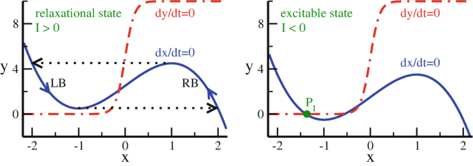

  

  The $\dot y=0$ (red dashed-dotted lines), and $\dot x=0$ (blue full lines) isocline of the Terman–Wang oscillator (9.39), here for $\alpha =5$, $\beta =0.2$, $\epsilon =0.1$. Left:$I=0.5$, shown is the relaxation cycle for $\epsilon \ll 1$ (dotted line, arrows). Right:$I=-0.5$, which has a stable fixpoint, $P_I$ (filled green dot)

• For $I<0$ and $|I|$ large enough, two additional fixpoints show up, as given by the crossing of the sigmoid $\alpha \big (1+\tanh (x/\beta )\big )$ with the left branch (LB) of the cubic $f(x)=3x-x^3+2$. One of the new fixpoints is stable.

The stable fixpoint $P_I$ is indicated in Fig. 9.7.

• Relaxation Regime

  For the $I>0$ the Terman–Wang oscillator relaxes to a periodic solution, see Fig. 9.7, which is akin to the relaxation oscillation observed for the Van der Pol oscillator.¹³

• Excitable State

  For $I<0$ the system settles into a stable fixpoint, becoming however active again when an external input shifts I into positive region. The system is said to be “excitable”.

The presence of an excitable state is a precondition for neuronal models.

Silent and Active Phases

In the relaxation regime, the periodic solution jumps rapidly, for $\epsilon \ll 1$, between trajectories that approach closely the right branch (RB), and the left branch (LB) of the $\dot x=0$ isocline. The times spent respectively on the two branches may however differ substantially, as indicated in Figs. 9.7 and 9.8. Indeed, the limit cycle is characterized by two distinct types of flows.

• Silent Phase

  Fig. 9.8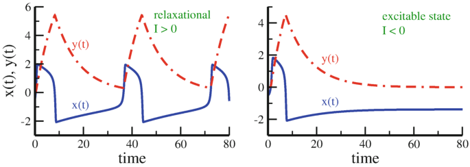

  

  Sample trajectories of $x(t)$ (blue line) and $y(t)$ (dashed-dotted line). Results for the Terman–Wang oscillator (9.39), together with $\alpha =5$, $\beta =0.2$, $\epsilon =0.1$. Left: Spiking behavior for $I=0.5$, characterized by silent/active phases for negative/positive x. Right: Relaxation to a stable fixpoint for $I=-0.5$

  The LB ($x<0$) of the $\dot x=0$ isocline is comparatively close to the $\dot y=0$ isocline, the system spends therefore considerable time on the LB. This leads to a “silent phase”, which is equivalent to a refractory period.

• Active Phase

  The RB ($x>0$) of the $\dot x=0$ isocline is far from the $\dot y=0$ isocline, when $\alpha \gg 1$, see Fig. 9.7. The time development $\dot y$ is hence fast on the RB, which defines the “active phase”.

The relative rate of the time development through $\dot y$ between silent and active phase is determined by the parameter $\alpha$, as defined in (9.39).

Spikes as Activity Bursts

In its relaxation phase, the Terman–Wang oscillator can be considered as a spontaneously spiking neuron, see Fig. 9.8. When $\alpha \gg 1$, the active phase undergoes a compressed burst, viz a “spike”.

The differential equation defined in (9.39) are examples of a standard technique within dynamical systems theory, the coupling of a slow variable to a fast variable, which results in a separation of time scales. When the slow variable $y=y(t)$ relaxes below a certain threshold, see Fig. 9.8, the fast variable $x=x(t)$ responds rapidly, resetting on the way the slow variable.

Synchronization via Fast Threshold Modulation

Limit cycle oscillators can synchronize, albeit slowly, via a common molecular field, as discussed in Sect. 9.2. Substantially faster synchronization can be achieved for networks of interacting relaxation oscillators via “fast threshold synchronization”.

The idea is simple. Relaxation oscillators are characterized by distinct phases during their cycle, which we denoted respectively silent and active states. These two states take functionally distinct roles when assuming that a neural oscillator is able to influence the threshold I of other units during its active phase, namely by emitting a short burst of activity, viz by spiking. For our basic equations (9.39), this concept translates into

$$\displaystyle \begin{aligned} I \to I + \varDelta I, \qquad \quad \varDelta I > 0\,, \end{aligned}$$

such that the second neural oscillator changes from an excitable state to the oscillating state. This process is illustrated graphically in Fig. 9.9, it corresponds to a signal sent from the first to the second dynamical unit. In neural terms, when the first neuron fires, the second neuron follows suit.

Fig. 9.9

Fast threshold modulation for two excitatory coupled relaxation oscillators, see (9.39), denoted symbolically as $o_1=o_1(t)$ and $o_2=o_2(t)$. When $o_1$ jumps at $t=t_1$ from the LB to the RB, it becomes active. The cubic $\dot x=0$ isocline for $o_2$ is consequently raised from C to $C_E$. This induces $o_2$ to jump as well from left to right. Note that the jumping from the right branch ($\mathrm {RB}$ and $\mathrm {RB}_E$) back to the left branches occurs in the reverse order, $o_2$ jumps first

Activity Propagation

A basic model illustrating the propagation of activity is given by a line of $i=1,\ldots ,N$ coupled oscillators $(x_i(t),y_i(t))$,

which are assumed to be initially all in the excitable state, with $I_i\equiv -0.5$. Inter-unit coupling via fast threshold modulation corresponds to

$$\displaystyle \begin{aligned} \varDelta I_i(t) = \varTheta(x_{i-1}(t))\,, {} \end{aligned} $$

(9.40)

where $\varTheta (x)$ is the Heaviside step function. That is, we define an oscillator i to be in its active phase whenever $x_i>0$. The resulting dynamics is shown in Fig. 9.10. The chain is driven by setting the first oscillator of the chain into the spiking state for a certain period of time. All other oscillators spike consecutively in rapid sequence.

Fig. 9.10

As an example of synchronization via causal signaling, shown are sample trajectories $x_i(t)$ (lines) for a line of coupled Terman–Wang oscillators, as defined by (9.39). The relaxation oscillators are in excitable states, with $\alpha =10$, $\beta =0.2$, $\epsilon =0.1$ and $I=-0.5$. For $t\in [20,100]$ a driving current $\varDelta I_1=1$ is added to the first oscillator (dotted line). In consequence, $x_1$ starts to spike, driving the other oscillators one by one via fast threshold modulation

9.5 Piecewise Linear Dynamical Systems

For an understanding of a dynamical system of interest, it is often desirable to study a simplified version. A standard technique involves to approximate non-linearities in the flow by piecewise linear functions. This technique allows at times to obtain analytic expressions for the orbits, which is a highly non-trivial outcome. For the case of limit-cycle oscillators, this approach can be carried out for our reference system, as defined by (9.39).

Piecewise Linear Terman–Wang Oscillators

We approximate the nullclines of (9.39) as

$$\displaystyle \begin{aligned} f(x) \to \left\{\begin{array}{rcl} 1-x &\ \mathrm{for}\ & x>0 \\ -1-x &\ \mathrm{for}\ & x<0 \end{array}\right., \qquad \quad g(x) \to \left\{\begin{array}{rcl} g_0 &\ \mathrm{for}\ & x>0 \\ -g_0 &\ \mathrm{for}\ & x<0 \end{array}\right.\,, {} \end{aligned} $$

(9.41)

as illustrated in Fig. 9.11. No fixpoint exists when $g_0>1$. In comparison to the original functionality shown in Fig. 9.7, the $\dot {x}=0$ and $\dot {y}=0$ isoclines are now discontinuous, but otherwise piecewise linear or constant functions.

Fig. 9.11

The piecewise linear Terman–Wang system, as described by (9.41) and (9.42). The parameters are $g_0\!=\!1.2$ and $\epsilon \!=\!1$. Left: The phase space $(x,y)$. Shown are the piecewise linear $\dot {x}\!=\!0$ isocline (blue), the piecewise constant $\dot {y}\!=\!0$ isolcine (red), and the resulting limit cycle (black). Right: As a function of time, kinks show up when the orbit crosses $x\!=\!0$. Compare Figs. 9.7, and 9.8

Piecewise Linear Dynamics

With $I\,{=}\,0$, the system becomes inversion symmetric. It is then sufficient to consider with

$$\displaystyle \begin{aligned} \dot{x} = 1-x-y, \qquad \quad \dot{y}= \epsilon(g_0-y) {} \end{aligned} $$

(9.42)

positive $x>0$. As a further simplification we set $\epsilon =1$. The solution of (9.42) takes the form

$$\displaystyle \begin{aligned} x = \big(\tilde{x}-\tilde{y}t\big)\mathrm{e}^{-t} + 1-g_0, \qquad \quad y = \tilde{y}\mathrm{e}^{-t} + g_0\,, {} \end{aligned} $$

(9.43)

which can be verified by direct differentiation. The trajectory is determined by three free parameters, $\tilde {x}$/$\tilde {y}$ and the yet unkown period T of the limit cycle.

Matching Conditions

The individual segments of a piecewise linear system need to be joined once explicit expressions for the solutions have been found. The resulting “matching conditions” determine the parameters appearing in the respective analytic solution.

Starting at $x(0)=0$, the orbit crosses the $x=0$ line the next time after half-a-period, which is evident from Fig. 9.11, with the y-component changing in between. The matching conditions are therefore

$$\displaystyle \begin{aligned} x(0)=0=x(T/2), \qquad \quad y(T/2) = - y(0)\,. {} \end{aligned} $$

(9.44)

The starting condition $x(0)=0$ yields $\tilde {x}=g_0-1$, see (9.43), which leads to

$$\displaystyle \begin{aligned} \begin{array}{rcl} g_0-1 & =&\displaystyle \Big(g_0-1-\tilde{y}\frac{T}{2}\Big) \,\mathrm{e}^{-T/2}, \\ 2g_0 & =&\displaystyle -\tilde{y} \big[ \mathrm{e}^{-T/2}+1\big]\,. {} \end{array} \end{aligned} $$

(9.45)

As a result one has two condition for two parameters, $\tilde {y}$ and T.

Limit Cycle Period

Given $g_0$, the only free model parameter, one can eliminate either $\tilde {y}$ or T from (9.45). Doing so, one obtains a self-consistency equation for the remaining parameter that can be solved numerically.

Alternatively we may ask which $g_0$ would lead to a given period T. In this case T is fixed und one eliminates $\tilde {y}$. From

$$\displaystyle \begin{aligned} \tilde{y} = \frac{2}{T}\left[1-\mathrm{e}^{T/2}\right](g_0-1), \qquad \quad \tilde{y}\left[1+\mathrm{e}^{-T/2}\right]= -2g_0 \end{aligned}$$

one finds

$$\displaystyle \begin{aligned} -2g_0=\frac{2}{T}(g_0-1) \left[1-\mathrm{e}^{T/2}\right] \left[1+\mathrm{e}^{-T/2}\right] \end{aligned}$$

and hence

$$\displaystyle \begin{aligned} g_0 = \frac{2\sinh(T/2)}{2\sinh(T/2)-T}\,, {} \end{aligned} $$

(9.46)

a remarkably simple expression. E.g., the orbit shown in Fig. 9.11 has a period of $T\approx 7.6$, which is consistent with $g_0=1.2,$.

Slow/Fast Oscillations

The advantage of an analytic result is that it allows to study limiting behaviors. On the positive y-axis, the orbit has to cross $x=0$ in the interval $[1,g_0]$, as evident from Fig. 9.11, given that $y=1$ and $y=g_0$ mark the upper/lower border of respectively the $\dot {x}=0$ and $\dot {y}=0$ isoclines. From (9.46) one finds

$$\displaystyle \begin{aligned} \lim_{T\to\infty} g_0 = 1\,, {} \end{aligned} $$

(9.47)

an expected relation. The oscillatory behavior slows down progressively when $g_0\to 1$, viz when the orbit needs to squeeze through the closing gap between the two isoclines. In the opposite limit, when $T\to 0$, the Taylor expansion $\sinh (z)\approx z + z^3/6$ leads to

$$\displaystyle \begin{aligned} g_0 \sim \frac{3}{T^2}, \qquad \quad T \sim \sqrt{\frac{3}{g_0}}, \qquad \quad T\ll 1\,. {} \end{aligned} $$

(9.48)

The flow accelerates as $1/\sqrt {g_0}$ when $g_0$ becomes large.

9.6 Synchronization Phenomena in Epidemics

There are illnesses, like measles, that come and go recurrently. Looking at the statistics of local measle outbreaks presented in Fig. 9.12, one can observe that outbreaks may occur in quite regular time intervals within a given city. Interestingly though, these outbreaks can be either in phase (synchronized) or out of phase between different cities.

Fig. 9.12

Observation of the number of infected persons in a study on illnesses. Top: Weekly cases of measle cases in Birmingham and Newcastle (red/blue lines). Bottom: Weekly cases of measle cases in Cambridge and Norwich (green/brown lines). Data from He and Stone (2003)

The oscillations in the number of infected persons are definitely not harmonic, sharing instead many characteristics with relaxation oscillations, which typically have silent and active phases, compare Sect. 9.4.2.

SIRS Model

The reference model for infectious diseases is the SIRS model. It contains three compartments, in the sense that individuals belong at any point in time to one of three possible classes.

$\begin {array}{rcl} \mathrm {S} & : & \mathrm {susceptible,}\\[0.1ex] \mathrm {I} & : & \mathrm {infected,}\\[0.1ex] \mathrm {R} & : & \mathrm {recovered.}\\ \end {array} \qquad \quad \qquad \quad \qquad \quad$

The dynamics is governed by the following rules:

• Infection Process

  With a certain probability, susceptibles pass to the infected state after coming into contact with one infected individual.

• Recovering

  Infected individuals recover from the infection after a given period of time, $\tau _I$, passing to the recovered state.

• Immunity

  For a certain period, $\tau _R$, recovered individuals are immune, returning to the susceptible state once when immunity is lost.

These three steps complete the infection circle $\mathrm {S}\to \mathrm {I} \to \mathrm {R} \to \mathrm {S}$. When $\tau _R\to \infty$ (lifelong immunity) the model reduces to the SIR-model.

Sum Rule

The SIRS model can be implemented both for discrete and for continuous time, we start with the former. The infected phase is normally short, which allows to use $\tau _I$ as the unit of time, setting $\tau _I=1$. The recovery time $\tau _R$ is then a multiple of $\tau _I=1$. We define with

• $x_t$ the fraction of infected individuals at time $t=1,2,3,\ldots$, and with

• $s_t$ the percentage of susceptible individuals at time t.

Normalizing the total number of individuals to one, the sum rule

$$\displaystyle \begin{aligned} s_t = 1 - x_t - \sum_{k=1}^{\tau_R} x_{t-k} = 1 - \sum_{k=0}^{\tau_R} x_{t-k} {} \end{aligned} $$

(9.49)

holds, as the fraction of susceptible individuals is just one minus the number of infected individuals minus the number of individuals in the recovery state, compare Fig. 9.13.

Fig. 9.13

Example of the course of an individual infection within the discrete-time SIRS model with an infection period $\tau _I=1$ and a recovery duration $\tau _R=3$. The number of individuals recovering at time t is the sum of infected individuals at times $t-1$, $t-2$ and $t-3$, compare (9.49)

Discrete Time SIRS Model

We denote with a the rate of transmitting an infection when there is a contact between an infected individual and a susceptible individual. Using the recursion relation (9.49) one obtains with

$$\displaystyle \begin{aligned} x_{t+1} = ax_ts_t = ax_t \left(1-\sum_{k=0}^{\tau_R} x_{t-k}\right) {} \end{aligned} $$

(9.50)

the discrete-time SIRS model.

Relation to the Logistic Map

For $\tau _R=0$, the discrete time SIRS model (9.50) reduces to the logistic map,

$$\displaystyle \begin{aligned} x_{t+1} = a x_t\left(1-x_t\right)\,. \end{aligned}$$

The trivial fixpoint $x_t\equiv 0$ is globally attracting when $a<1$, which implies that the illness dies out. The non-trivial steady state is

$$\displaystyle \begin{aligned} x^{(1)} = 1-\frac{1}{a}, \qquad \quad \mathrm{for} \quad 1<a<3\,. \end{aligned}$$

At $a=3$ a Hopf bifurcation is observed, beyond an oscillation of period two. Increasing the growth rate a further, a transition to deterministic chaos takes place.

The SIRS model (9.50) shows somewhat similar behaviors. Due to the memory terms $x_{t-k}$, the resulting oscillations may however depend on the initial condition. For extended immunities, $\tau _R\gg \tau _I$, features characteristic of relaxation oscillators are found, compare Fig. 9.14.

Fig. 9.14

Example of a solution to the SIRS model, see (9.50), for $\tau _R=6$. The number of infected individuals might drop to very low values during the silent phase in between two outbreaks, as most of the population is first infected and then immunized during an outbreak

Two Coupled Epidemic Centers

What happens when two epidemic centers are weakly coupled? We use

$$\displaystyle \begin{aligned} s_t^{(1,2)}, \qquad \quad x_t^{(1,2)} \end{aligned}$$

to denote the fraction of susceptible/infected individuals in the respective cities. Different dynamical couplings are conceivable, via exchange or visits of susceptible or infected individuals. With

$$\displaystyle \begin{aligned} \begin{array}{rcl} x_{t+1}^{(1)} & =&\displaystyle a\left(x_t^{(1)}+e\,x_t^{(2)}\right)s_t^{(1)}, \\[0.5ex] x_{t+1}^{(2)} & =&\displaystyle a\left(x_t^{(2)}+e\,x_t^{(1)}\right)s_t^{(2)}\,, {} \end{array} \end{aligned} $$

(9.51)

one describes a situation where a small fraction e of infected individuals visits the respective other center. In addition, one needs to apply the sum rule (9.49) to both centers.

For $e=1$ there is no distinction between the two centers, which means that the dynamics described by (9.51) can be merged via $x_t=x_t^{(1)}+x_t^{(2)}$ and $s_t=s_t^{(1)}+s_t^{(2)}$. A single combined epidemic population remains. The situation is similar to the case of to coupled logistic maps, as given by (9.37). This is not surprising, since the coupling term in (9.51) is based on aggregate averaging.

In Phase Versus Out of Phase Synchronization

We have seen in Sect. 9.2, that relaxation oscillators coupled strongly during their active phases synchronize rapidly. Here the active phase corresponds to an outbreak of the illness, which is however not pre-given, but a self-organized event. In this sense one implements with (9.51) a coupling equivalent to a fast threshold modulation, as discussed in Sect. 9.4.2, albeit based on a self-organized process.

In Fig. 9.15 we present the results from a numerical simulation of the coupled model, illustrating the typical behavior. We see that the epidemic outbreaks occur in the SIRS model indeed in phase for moderate to large coupling constants e. In contrast, for very small couplings e between the two centers of epidemics, the synchronization phase flips to antiphase. This phenomenon is observed in reality, compare Fig. 9.12.

Fig. 9.15

Time evolution of the fraction of infected individuals $x^{(1)}(t)$ and $x^{(2)}(t)$ within the SIRS model, see (9.51), for two epidemic centers $i=1,2$ with recovery times $\tau _R=6$ and infection rates $a=2$, see (9.50). For a very weak coupling $e=0.005$ (top) the outbreaks occur out of phase, for a moderate coupling $e=0.1$ (bottom) in phase

Time Scale Separation

The reason for the occurrence of out of phase synchronization is the emergence of two separate time scales in the limit $t_R\gg 1$ and $e\ll 1$. A small seed ${\sim }e a x^{(1)} s^{(2)}$ of infections in the second city needs substantial time to induce a full-scale outbreak, even via exponential growth, when e is too small. But in order to remain in phase with the current outbreak in the first city the outbreak occurring in the second city may not lag too far behind. When the dynamics is symmetric under exchange $1\leftrightarrow 2$ the system then settles in antiphase cycles.

9.6.1 Continuous Time SIRS Model

Changing notation slightly, we use S, I, and $R=1-I-S$ for the densities of susceptible, infected, and recovered.

Continuous Time Limit

Substituting the discrete-time approximation for the derivative,

$$\displaystyle \begin{aligned} \dot{I}\approx \frac{I_{t+\varDelta t}-I_t}{\varDelta t}, \qquad \quad \varDelta t = 1\,, \end{aligned}$$

in (9.50) yields

$$\displaystyle \begin{aligned} \dot I = aI(1-I-R) - I = aIS - I\,, {} \end{aligned} $$

(9.52)

which has a simple interpretation. The number of infected increases with a rate that is proportional to the infection probability a and to the densities I and S of infected and susceptibles. The term $-I$ describes per-time recovering.

Continuous Time SIRS Model

For the discrete case, we took the duration of the illness as the unit of time, as illustrated in Fig. 9.13. Using (9.52) and rescaling time by $T=1/\lambda$, one obtains with

$$\displaystyle \begin{aligned} \dot{S} = -gIS + \delta R, \qquad \quad \dot{I} = gIS -\lambda I, \qquad \quad \dot{R} = +\lambda I - \delta R {} \end{aligned} $$

(9.53)

the standard continuous time SIRS model, where $g=\lambda a$ and $\delta = \lambda /\tau _R$. Recall that $\tau _R$ denotes the average time an individual remains immune, as measured in units of illness duration T.

Endemic Fixpoint

The endemic state is defined by the fixpoint condition

$$\displaystyle \begin{aligned} S = \frac{\lambda}{g}, \qquad \quad I = \frac{g-\lambda}{\delta+\lambda}, \qquad \quad R = \frac{\lambda}{\delta}\, \frac{g-\lambda}{\delta+\lambda}\,, {} \end{aligned} $$

(9.54)

which follows directly from (9.53). It exists when the infection rate g is larger than the recovery rate $\lambda$, namely when $g>\lambda$. Otherwise, the illness dies out. One can show that the endemic state is always stable. The discrete SIRS model supports in contrast solutions corresponding to periodic outbreaks, as shown in Fig. 9.13.

Analytic Solution of the SIR Model

Life-long immunity, which corresponds to setting $\delta =0$ in (9.53), reduces the SIRS model to the SIR model. Dividing the equation for $\dot {I}$ by the one for $\dot {S}$ yields

$$\displaystyle \begin{aligned} \frac{\dot{I}}{\dot{S}} = \frac{dI}{dS} = -1 + \frac{\lambda}{g}\,\frac{1}{S}\,, {} \end{aligned} $$

(9.55)

which has the solution

$$\displaystyle \begin{aligned} I(t) = 1-R_0-S(t) + \frac{\lambda}{g}\, \log\left(\frac{S(t)}{S_0}\, \right)\,, {} \end{aligned} $$

(9.56)

where $S_0=S(0)$, $I_0=I(0)$ and $R_0=1-S_0-I_0$ denote the starting configuration. The functional dependence of $I=I(X)$ is shown in Fig. 9.16, where $X=I+R=1-S$ is the cumulative number of cases. The illness dies out before the entire population has been infected.

Fig. 9.16

For the SIR model, the current number of infected I as a function of the cumulative number of cases $X=1-S$. The curves are described by the analytic solution (9.56), using $R_0=0=I_0$ and $S_0=1$. The outbreak starts at $(X,I)=(0,0)$, ending when I vanishes again (open circles). A sizeable fraction of the population is never infected

Exercises

• (9.1) The Driven Harmonic Oscillator

  Solve the driven harmonic oscillator, see (9.1), for all times t and compare it with the long time solution $t\to \infty$, Eqs. (9.3) and (9.4).

• (9.2) Self-Synchronization

  Consider an oscillator with time delay feedback,

  $$\displaystyle \begin{aligned} \dot\theta(t) = \omega_0 + K\sin[\theta(t-T)-\theta(t)]\,. \end{aligned}$$

  Discuss the self-synchronization in analogy to the stability of the steady-state solutions of time delay systems.¹⁴ Which is the auto-locking frequency in the limit of strong self-coupling, $K\to \infty$?

• (9.3) Kuramoto model with three oscillators

  Consider the Kuramoto model, as defined by (9.5) and (9.6), for three identical oscillators. Start by showing that the natural frequencies can be disregarded when $\omega _i\equiv \omega$. Use relative variables $\alpha = \theta _2-\theta _1$ and $\beta = \theta _3-\theta _2$, for the determination of the fixpoints. Which ones are stable/unstable for $K>0$ and/or $K<0$?

• (9.4) Lyapunov Exponents along synchronized Orbits

  Evaluate, for two coupled oscillators, see (9.7), the longitudinal and the orthogonal Lyapunov exponents, with respect to the synchronized orbit. Does the average of the longitudinal Lyapunov exponent over one period vanish?

• (9.5) Synchronization of Chaotic Maps

  The Bernoulli shift map $f(x)=ax\ \mathrm {mod}\ 1$ with $x\in [0,1]$ is chaotic for $a>1$. Consider with

  $$\displaystyle \begin{aligned} \begin{array}{rcl} x_1(t+1) &=& f\big([1-\kappa]x_1(t)+\kappa x_2(t-T)\big) \\[0.5ex] x_2(t+1) &=& f\big([1-\kappa]x_2(t)+\kappa x_1(t-T)\big) \end{array} {} \end{aligned} $$

  (9.57)

  two coupled chaotic maps, with $\kappa \in [0,1]$ being the coupling strength and T the time delay, compare (9.32). Discuss the stability of the synchronized states $x_1(t)=x_2(t)\equiv \bar {x}(t)$ for general time delays T. What drives the synchronization process?

• (9.6) Terman–Wang Oscillator

  Discuss the stability of the fixpoints of the Terman–Wang oscillator, see (9.39). Linearize the differential equations around the fixpoint solution and consider the limit $\beta \to 0$.

• (9.7) Pulse Coupled Leaky Integrator Neurons

  The membrane potential $x(t)$ of a leaky-integrator neuron can be thought to increase over time like

  $$\displaystyle \begin{aligned} \dot x = \gamma(S_0-x), \qquad \quad x(t) = S_0\left(1-\mathrm{e}^{-\gamma t}\right)\,. {} \end{aligned} $$

  (9.58)

  When the membrane potential reaches a certain threshold, say $x_\theta =1$, it spikes and resets its membrane potential to $x\to 0$ immediately after spiking. For two pulse coupled leaky integrators $x_A(t)$ and $x_B(t)$ the spike of one neuron induces an increase in the membrane potential of the other neuron by a finite amount $\epsilon$. Discuss and find the limiting behavior for long times.

• (9.8) SIRS Model

  Find the fixpoints $x_t\equiv x^*$ of the discrete-time SIRS model, see (9.50), for all $\tau _R$. As a function of a, study the stability for $\tau _R=0,1$.

• (9.9) Epidemiology of Zombies

  If humans and zombies meet, there are only two possible outcomes. Either the zombie bites the human, or the human kills the zombie, Defining with $\alpha \in [0,1]$ and $1-\alpha$ the respective probabilities, the evolution equations for the two population densities H and Z are

  $$\displaystyle \begin{aligned} \dot{H} = -\alpha HZ, \qquad \quad \dot{Z} = (2\alpha-1) HZ\,. {} \end{aligned} $$

  (9.59)

  Find and discuss the analytic solution when starting from initial densities $H_0$ and $Z_0=1-H_0$. Which is the difference to the SIRS model?

Further Reading

The reader may consult a textbook containing examples for synchronization processes by Pikovsky et al. (2003), and an informative review of the Kuramoto model by Pikovsky and Rosenblum (2015), which contains in addition historical annotations. Some of the material discussed in this chapter requires a certain background in theoretical neuroscience, see e.g. Sterrat et. al (2023). An introductory review to chimera states is given in Panaggio and Abrams (2015).

We recommend that the interested reader takes a look at some of the original research literature, such as the exact solution relaxation oscillators, Terman and Wang (1995), the concept of fast threshold synchronization, Somers and Kopell (1993), the physics of synchronized clapping, Néda et al. (2000a,b), and synchronization phenomena within the SIRS model of epidemics, He and Stone (2003). For synchronization with delays see D’Huys et al. (2008).

References

D’Huys, O.,Vicente, R., Erneux, T., Danckaert, J., & Fischer, I. (2008). Synchronization properties of network motifs: Influence of coupling delay and symmetry. Chaos, 18, 037116.
He, D., & Stone, L. (2003). Spatio-temporal synchronization of recurrent epidemics. Proceedings of the Royal Society London B, 270, 1519–1526.
Néda, Z., Ravasz, E., Vicsek, T., Brechet, Y., & Barabási, A. L. (2000a). Physics of the rhythmic applause. Physical Review E, 61, 6987–6992.
Néda, Z., Ravasz, E., Vicsek, T., Brechet, Y., & Barabási, A.L. (2000b). The sound of many hands clapping. Nature, 403, 849–850.
Panaggio, M. J., & Abrams, D. M. (2015). Chimera states: coexistence of coherence and incoherence in networks of coupled oscillators. Nonlinearity, 28, R67.
Pikovsky, A., & Rosenblum, B. (2015). Dynamics of globally coupled oscillators: Progress and perspectives. Chaos, 25, 9.
Pikovsky, A., Rosenblum, M., & Kurths, J. (2003). Synchronization: A universal concept in nonlinear sciences. Cambridge University Press.
Somers, D., & Kopell, N. (1993). Rapid synchronization through fast threshold modulation. Biological Cybernetics, 68, 398–407.
Sterratt, D., Graham, B., Gillies, A., Einevoll, G., & Willshaw, D. (2023). Principles of computational modelling in neuroscience. Cambridge University Press.
Strogatz, S. H. (2001). Exploring complex networks. Nature, 410, 268–276.
Terman, D., & Wang, D. L. (1995) Global competition and local cooperation in a network of neural oscillators. Physica D, 81, 148–176.
Author information
Authors and Affiliations
Rights and permissions
Copyright information
© 2024 The Author(s), under exclusive license to Springer Nature Switzerland AG
About this chapter
Cite this chapter
Gros, C. (2024). Synchronization Phenomena. In: Complex and Adaptive Dynamical Systems. Springer, Cham. https://doi.org/10.1007/978-3-031-55076-8_9
Download citation
DOI: https://doi.org/10.1007/978-3-031-55076-8_9
Published:
Publisher Name: Springer, Cham
Print ISBN: 978-3-031-55075-1
Online ISBN: 978-3-031-55076-8
eBook Packages: Physics and AstronomyPhysics and Astronomy (R0)